Financial Models

The financial problems model is divided into two parts:

1. The financial model
2. The function that acts on this model

See the examples below.

Example 1 - Quantum Risk Analysis

Risk analysis aims to evaluate the potential for loss in an investment. Specifically, an investor needs to quantify how large a loss on investment could be, given a certain level of confidence, over a period of time. This quantity is known as the value at risk (VaR). The VaR is based on the statistical characteristics of the investment and the shape of its distribution curve. It is evaluated using intensive computations of the aggregated value for M different realizations of portfolio assets model. The width of the confidence interval scales like \(O(M^{-1/2})\). To calculate the VaR of an assets portfolio on a quantum computer, define the VaR such that [1] .

\[ VaR = argmin_{x_0}{(P(x > x_0) <= \alpha)} \]

where \(x \in {0,...N-1}\) and \(\alpha\) is the confidence level, i.e., the percentage that a loss is larger than the VaR. The VaR is the smallest value of x with a confidence level of \(\alpha\).

To create a quantum program that can solve this kind of problem:

1. Create a distribution function that represents the assets portfolio.
2. Construct the VaR operator.
3. Extract the VaR using amplitude estimation.

Use the Classiq financial package to do this in two phases:

1. {==Financial model==} which contains the distribution function.
2. {==Financial function==} \(f_x(i)\) that is implemented by the model.

Financial Model

In our example, the model is a Gaussian model (called Conditioned Gaussian) of a two-asset portfolio.

The parameters that define this model:

• num qubits (int): Number of qubits that describe the accuracy of the Gaussian
• normal max value (float): The discrete number where the Gaussian is truncated
• default probabilities (List[float]): The loss probability of each asset
• rhos (List[float]): The width of the Gaussian
• loss (List[int]): The loss of each asset
• min loss (int): The minimum loss of the entire distribution

Financial Function

On the same financial model, you can generate several quantum programs with different financial functions. The current example generates the VaR function.

The parameters for the finance function:

• f: The finance function type
• condition:
• threshold: threshold to use the function. otherwise it's 0.
• larger: whether the threshold is from beneath or above.

Full Example

In the next example, we will demonstrate how to extract the CDF value of a given value x for a given probability distribution. That can be used to extract the Var of the distribution, using a bisection search.

IDESDK

Synthesizing a Financial Model

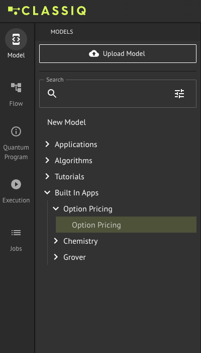
In the IDE Model page: select Option Pricing from the Built In Apps folder in the Models pane:

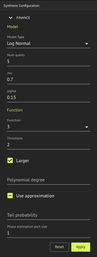
By modifying the Finance model editor pane and then clicking the Apply button, the model is populated in the Model Editor pane.

Pressing the Synthesize button generates the quantum program and shows its graphical representation.

Executing the Quantum Program

The synthesized quantum program can be executed from the execution section of the IDE or from the SDK (see execution).

To execute from within the IDE, select Execute button from the Quantum Program page.

from classiq import (
    construct_finance_model,
    synthesize,
    execute,
    set_constraints,
    Constraints,
)
from classiq.applications.finance import function_input, gaussian_model_input

gaussian_model = gaussian_model_input.GaussianModelInput(
    num_qubits=2,
    normal_max_value=2,
    default_probabilities=[0.15, 0.25],
    rhos=[0.1, 0.05],
    loss=[1, 2],
    min_loss=0,
)

condition = function_input.FunctionCondition(threshold=2, larger=True)
finance_function = function_input.FinanceFunctionInput(
    f="var",
    condition=condition,
)

model = construct_finance_model(
    finance_model_input=gaussian_model,
    finance_function_input=finance_function,
    phase_port_size=2,
)

model = set_constraints(model, Constraints(max_width=10))

quantum_program = synthesize(model)
results = execute(quantum_program).result()
print(results[0].name, ":", results[0].value)

This is the output quantum program, with some (but not all) of its blocks expanded:

This program can be executed on a quantum computer.

Example 2 - Option Pricing

An option is the possibility to buy (call) or sell (put) an item (or share) at a known price: the strike price (K). The option has a maturity price (S). The payoff function to describe, for example, a European call option, is this:

\[ \Bigg\{\begin{array}{lr} 0, & \text{when } K\geq S\\ S - K, & \text{when } K < S\end{array} \]

The maturity price is unknown, therefore it is expressed by a price distribution function, which may be any type of distribution function. For example, a log-normal distribution: \(X=e^{\mu+\sigma Z}\), where \(\mu,\sigma\) are the mean and STD respectively and Z is the standard normal distribution.

To estimate the option price using a quantum computer:

1. Load the wanted distribution, that is, discretize the distribution using \(2^n\) points (where n is the number of qubits) and truncate it.
2. Implement the payoff function that is equal to zero if \(S\leq{K}\) and increases linearly. The linear part is approximated to load it properly using \(R_y\) rotations [3] .
3. Evaluate the expected payoff using amplitude estimation.

In this case, the threshold argument refers to the strike price \(K\), and we look for the case where the maturity price (\(S\)) is larger than the strike price (putting it to True). The phase_port_size determines the number of qubits used by the phase estimation algorithm (implemented inside the amplitude estimation algorithm) that sets the accuracy of the calculation. In other words, more qubits lead to a more accurate solution with a price of bigger quantum programs.

The result shows the expected value of the payoff function according to the given probability distribution.

Models

The available models on the Classiq platform:

• gaussian - abbreviation of 'Gaussian conditional independence model'
• log normal

Functions

The available functions:

• var
• expected shortfall
• european call option
• x**2

References

[1] Woerner, S., Egger, D.J. Quantum risk analysis. npj Quantum Inf 5, 15 (2019).