Set Cover Problem
Introduction
The set cover problem [1] represents a well-known problem in the fields of combinatorics, computer science, and complexity theory. It is an NP-complete problems.
The problem presents us with a universal set, \(\displaystyle U\), and a collection \(\displaystyle S\) of subsets of \(\displaystyle U\). The goal is to find the smallest possible subfamily, \(\displaystyle C \subseteq S\), whose union equals the universal set.
Formally, let's consider a universal set \(\displaystyle U = {1, 2, ..., n}\) and a collection \(\displaystyle S\) containing \(m\) subsets of \(\displaystyle U\), \(\displaystyle S = {S_1, ..., S_m}\) with \(\displaystyle S_i \subseteq U\). The challenge of the set cover problem is to find a subset \(\displaystyle C\) of \(\displaystyle S\) of minimal size such that \(\displaystyle \bigcup_{S_i \in C} S_i = U\).
Solving with the Classiq platform
We go through the steps of solving the problem with the Classiq platform, using QAOA algorithm [2]. The solution is based on defining a pyomo model for the optimization problem we would like to solve.
Building the Pyomo model from an input
We proceed by defining the pyomo model that will be used on the Classiq platform, using the mathematical formulation defined above:
import itertools
from typing import List

import pyomo.core as pyo


def set_cover(sub_sets: List[List[int]]) -> pyo.ConcreteModel:
    entire_set = set(itertools.chain(*sub_sets))
    n = max(entire_set)
    num_sets = len(sub_sets)
    assert entire_set == set(
        range(1, n + 1)
    ), f"the union of the subsets is {entire_set} not equal to range(1, {n + 1})"

    model = pyo.ConcreteModel()
    model.x = pyo.Var(range(num_sets), domain=pyo.Binary)

    @model.Constraint(entire_set)
    def independent_rule(model, num):
        return sum(model.x[idx] for idx in range(num_sets) if num in sub_sets[idx]) >= 1

    model.cost = pyo.Objective(expr=sum(model.x.values()), sense=pyo.minimize)

    return model
The model contains:
-
Binary variable for each subset (model.x) indicating if it is included in the sub-collection.
-
Objective rule – the size of the sub-collection.
-
Constraint – the sub-collection covers the original set.
sub_sets = sub_sets = [
    [1, 2, 3, 4],
    [2, 3, 4, 5],
    [6, 7],
    [8, 9, 10],
    [1, 6, 8],
    [3, 7, 9],
    [4, 7, 10],
    [2, 5, 8],
]

set_cover_model = set_cover(sub_sets)
set_cover_model.pprint()
1 Var Declarations
    x : Size=8, Index={0, 1, 2, 3, 4, 5, 6, 7}
        Key : Lower : Value : Upper : Fixed : Stale : Domain
          0 :     0 :  None :     1 : False :  True : Binary
          1 :     0 :  None :     1 : False :  True : Binary
          2 :     0 :  None :     1 : False :  True : Binary
          3 :     0 :  None :     1 : False :  True : Binary
          4 :     0 :  None :     1 : False :  True : Binary
          5 :     0 :  None :     1 : False :  True : Binary
          6 :     0 :  None :     1 : False :  True : Binary
          7 :     0 :  None :     1 : False :  True : Binary

1 Objective Declarations
    cost : Size=1, Index=None, Active=True
        Key  : Active : Sense    : Expression
        None :   True : minimize : x[0] + x[1] + x[2] + x[3] + x[4] + x[5] + x[6] + x[7]

1 Constraint Declarations
    independent_rule : Size=10, Index={1, 2, 3, 4, 5, 6, 7, 8, 9, 10}, Active=True
        Key : Lower : Body               : Upper : Active
          1 :   1.0 :        x[0] + x[4] :  +Inf :   True
          2 :   1.0 : x[0] + x[1] + x[7] :  +Inf :   True
          3 :   1.0 : x[0] + x[1] + x[5] :  +Inf :   True
          4 :   1.0 : x[0] + x[1] + x[6] :  +Inf :   True
          5 :   1.0 :        x[1] + x[7] :  +Inf :   True
          6 :   1.0 :        x[2] + x[4] :  +Inf :   True
          7 :   1.0 : x[2] + x[5] + x[6] :  +Inf :   True
          8 :   1.0 : x[3] + x[4] + x[7] :  +Inf :   True
          9 :   1.0 :        x[3] + x[5] :  +Inf :   True
         10 :   1.0 :        x[3] + x[6] :  +Inf :   True

3 Declarations: x independent_rule cost
Setting Up the Classiq Problem Instance
In order to solve the Pyomo model defined above, we use the CombinatorialProblem quantum object. Under the hood it tranlastes the Pyomo model to a quantum model of the QAOA algorithm, with a cost function translated from the Pyomo model. We can choose the number of layers for the QAOA ansatz using the argument num_layers, and the penalty_factor, which will be the coefficient of the constraints term in the cost hamiltonian.
from classiq import *
from classiq.applications.combinatorial_optimization import CombinatorialProblem

combi = CombinatorialProblem(pyo_model=set_cover_model, num_layers=3, penalty_factor=10)

qmod = combi.get_model()
Synthesizing the QAOA Circuit and Solving the Problem
We can now synthesize and view the QAOA circuit (ansatz) used to solve the optimization problem:
qprog = combi.get_qprog()
show(qprog)
Quantum program link: https://platform.classiq.io/circuit/39FjWgm2BVRqBIpje7e1f6HNrAf


https://platform.classiq.io/circuit/39FjWgm2BVRqBIpje7e1f6HNrAf?login=True&version=17
We now solve the problem by calling the optimize method of the CombinatorialProblem object. For the classical optimization part of the QAOA algorithm we define the maximum number of classical iterations (maxiter) and the \(\alpha\)-parameter (quantile) for running CVaR-QAOA, an improved variation of the QAOA algorithm [3]:
optimized_params = combi.optimize(maxiter=60, quantile=0.7)
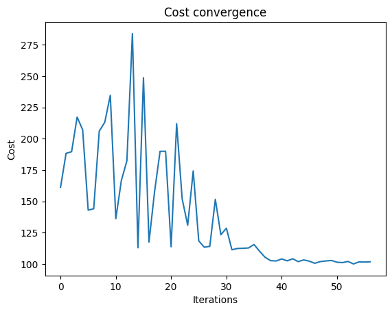
We can check the convergence of the run:
import matplotlib.pyplot as plt

fig, axes = plt.subplots(nrows=1, ncols=1)
axes.plot(combi.cost_trace)
axes.set_xlabel("Iterations")
axes.set_ylabel("Cost")
axes.set_title("Cost convergence")
Text(0.5, 1.0, 'Cost convergence')
Optimization Results
We can also examine the statistics of the algorithm. In order to get samples with the optimized parameters, we call the sample method:
optimization_result = combi.sample(optimized_params)
optimization_result.sort_values(by="cost").head(5)
| solution | probability | cost | |
|---|---|---|---|
| 52 | {'x': [0, 1, 0, 1, 1, 0, 0, 0], 'independent_r... | 0.001465 | 23.0 |
| 66 | {'x': [0, 1, 0, 1, 1, 0, 0, 0], 'independent_r... | 0.001465 | 23.0 |
| 1107 | {'x': [0, 1, 0, 0, 1, 0, 1, 0], 'independent_r... | 0.000488 | 23.0 |
| 636 | {'x': [1, 0, 1, 1, 0, 0, 0, 0], 'independent_r... | 0.000488 | 23.0 |
| 1531 | {'x': [0, 1, 0, 0, 1, 0, 1, 0], 'independent_r... | 0.000488 | 23.0 |
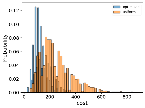
We also want to compare the optimized results to uniformly sampled results:
uniform_result = combi.sample_uniform()
And compare the histograms:
optimization_result["cost"].plot(
    kind="hist",
    bins=50,
    edgecolor="black",
    weights=optimization_result["probability"],
    alpha=0.6,
    label="optimized",
)
uniform_result["cost"].plot(
    kind="hist",
    bins=50,
    edgecolor="black",
    weights=uniform_result["probability"],
    alpha=0.6,
    label="uniform",
)
plt.legend()
plt.ylabel("Probability", fontsize=16)
plt.xlabel("cost", fontsize=16)
plt.tick_params(axis="both", labelsize=14)
Let us plot the solution:
best_solution = optimization_result.solution[optimization_result.cost.idxmin()]
best_solution = [best_solution["x"][i] for i in range(len(best_solution["x"]))]
best_solution
[0, 1, 0, 1, 1, 0, 0, 0]
print(
    f"Quantum Solution: num_sets={int(sum(best_solution))}, sets={[sub_sets[i] for i in range(len(best_solution)) if best_solution[i]]}"
)
Quantum Solution: num_sets=3, sets=[[2, 3, 4, 5], [8, 9, 10], [1, 6, 8]]
Comparison to a classical solver
Lastly, we can compare to the classical solution of the problem:
from pyomo.opt import SolverFactory

solver = SolverFactory("couenne")
solver.solve(set_cover_model)
classical_solution = [
    int(pyo.value(set_cover_model.x[i])) for i in range(len(set_cover_model.x))
]
print("Classical solution:", classical_solution)
Classical solution: [1, 1, 1, 1, 0, 0, 0, 0]
print(
    f"Classical Solution: num_sets={int(sum(classical_solution))}, sets={[sub_sets[i] for i in range(len(classical_solution)) if classical_solution[i]]}"
)
Classical Solution: num_sets=4, sets=[[1, 2, 3, 4], [2, 3, 4, 5], [6, 7], [8, 9, 10]]
References
[1]: Integer Programming (Wikipedia).
[2]: Farhi, Edward, Jeffrey Goldstone, and Sam Gutmann. "A quantum approximate optimization algorithm." arXiv preprint arXiv:1411.4028 (2014).
[3]: Barkoutsos, Panagiotis Kl, et al. "Improving variational quantum optimization using CVaR." Quantum 4 (2020): 256.