Max Independent Set
Introduction
In the Maximum Independent Set Problem [1], we need to find the largest subset of vertices in a given graph, such that no two vertices in the subset are adjacent. This is an NP-Hard problem in general graph structures, with applications in various fields such as network deign, bioinformatics, and scheduling.
Mathematical Formulation
Given a graph \(G=(V,E)\), an independent set \(I \subseteq V\) is a set of vertices such that no two vertices in \(I\) are adjacent. The Maximum Independent Set Problem is the problem of finding the independent set \(I\) with maximum cardinality. In binary form, we can represent each vertex \(v\) being in or out of the independent set \(I\) by a binary variable \(x_v\), with \(x_v = 1\) if \(v \in I\), and \(x_v = 0\) otherwise. The problem can then be formulated as:
Maximize \(\sum_{v \in V} x_v\)
Subject to:
\(x_{u} + x_{v} \leq 1, \forall (u, v) \in E\)
where each \(x_v \in {0,1}\).
Solving with the Classiq platform
We go through the steps of solving the problem with the Classiq platform, using QAOA algorithm [2]. The solution is based on defining a pyomo model for the optimization problem we would like to solve.
import networkx as nx
import numpy as np
import pyomo.core as pyo
from IPython.display import Markdown, display
from matplotlib import pyplot as plt
Building the Pyomo model from a graph input
We proceed by defining the pyomo model that will be used on the Classiq platform, using the mathematical formulation defined above:
def mis(graph: nx.Graph) -> pyo.ConcreteModel:
    model = pyo.ConcreteModel()
    model.x = pyo.Var(graph.nodes, domain=pyo.Binary)

    @model.Constraint(graph.edges)
    def independent_rule(model, node1, node2):
        return model.x[node1] + model.x[node2] <= 1

    model.cost = pyo.Objective(expr=sum(model.x.values()), sense=pyo.maximize)

    return model
The model consists of:
-
Index set declarations (model.Nodes, model.Arcs).
-
Binary variable declaration for each node (model.x) indicating whether that node is chosen to be included in the set.
-
Constraint rule - for each edge we require at least one of the corresponding node variables to be 0.
-
Objective rule – the sum of the variables equals to the set size.
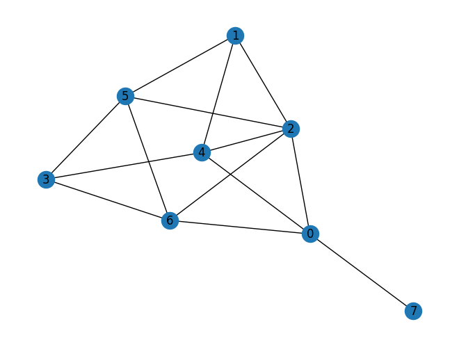
num_nodes = 8
p_edge = 0.4
graph = nx.fast_gnp_random_graph(n=num_nodes, p=p_edge, seed=12345)

nx.draw_kamada_kawai(graph, with_labels=True)
mis_model = mis(graph)
mis_model.pprint()
2 Set Declarations
    independent_rule_index : Size=1, Index=None, Ordered=False
        Key  : Dimen : Domain : Size : Members
        None :     2 :    Any :   14 : {(0, 2), (0, 4), (0, 6), (0, 7), (1, 2), (1, 4), (1, 5), (2, 4), (2, 5), (2, 6), (3, 4), (3, 5), (3, 6), (5, 6)}
    x_index : Size=1, Index=None, Ordered=False
        Key  : Dimen : Domain : Size : Members
        None :     1 :    Any :    8 : {0, 1, 2, 3, 4, 5, 6, 7}

1 Var Declarations
    x : Size=8, Index=x_index
        Key : Lower : Value : Upper : Fixed : Stale : Domain
          0 :     0 :  None :     1 : False :  True : Binary
          1 :     0 :  None :     1 : False :  True : Binary
          2 :     0 :  None :     1 : False :  True : Binary
          3 :     0 :  None :     1 : False :  True : Binary
          4 :     0 :  None :     1 : False :  True : Binary
          5 :     0 :  None :     1 : False :  True : Binary
          6 :     0 :  None :     1 : False :  True : Binary
          7 :     0 :  None :     1 : False :  True : Binary

1 Objective Declarations
    cost : Size=1, Index=None, Active=True
        Key  : Active : Sense    : Expression
        None :   True : maximize : x[0] + x[1] + x[2] + x[3] + x[4] + x[5] + x[6] + x[7]

1 Constraint Declarations
    independent_rule : Size=14, Index=independent_rule_index, Active=True
        Key    : Lower : Body        : Upper : Active
        (0, 2) :  -Inf : x[0] + x[2] :   1.0 :   True
        (0, 4) :  -Inf : x[0] + x[4] :   1.0 :   True
        (0, 6) :  -Inf : x[0] + x[6] :   1.0 :   True
        (0, 7) :  -Inf : x[0] + x[7] :   1.0 :   True
        (1, 2) :  -Inf : x[1] + x[2] :   1.0 :   True
        (1, 4) :  -Inf : x[1] + x[4] :   1.0 :   True
        (1, 5) :  -Inf : x[1] + x[5] :   1.0 :   True
        (2, 4) :  -Inf : x[2] + x[4] :   1.0 :   True
        (2, 5) :  -Inf : x[2] + x[5] :   1.0 :   True
        (2, 6) :  -Inf : x[2] + x[6] :   1.0 :   True
        (3, 4) :  -Inf : x[3] + x[4] :   1.0 :   True
        (3, 5) :  -Inf : x[3] + x[5] :   1.0 :   True
        (3, 6) :  -Inf : x[3] + x[6] :   1.0 :   True
        (5, 6) :  -Inf : x[5] + x[6] :   1.0 :   True

5 Declarations: x_index x independent_rule_index independent_rule cost
Setting Up the Classiq Problem Instance
In order to solve the Pyomo model defined above, we use the CombinatorialProblem python class. Under the hood it tranlates the Pyomo model to a quantum model of the QAOA algorithm, with cost hamiltonian translated from the Pyomo model. We can choose the number of layers for the QAOA ansatz using the argument num_layers.
from classiq import *
from classiq.applications.combinatorial_optimization import CombinatorialProblem

combi = CombinatorialProblem(pyo_model=mis_model, num_layers=3)

qmod = combi.get_model()
write_qmod(qmod, "max_independent_set")
Synthesizing the QAOA Circuit and Solving the Problem
We can now synthesize and view the QAOA circuit (ansatz) used to solve the optimization problem:
qprog = combi.get_qprog()
show(qprog)
Opening: https://platform.classiq.io/circuit/2v4c6BmZR7F3HBXDnOj9ZWVDECt?login=True&version=0.73.0
We now solve the problem by calling the optimize method of the CombinatorialProblem object. For the classical optimization part of the QAOA algorithm we define the maximum number of classical iterations (maxiter) and the \(\alpha\)-parameter (quantile) for running CVaR-QAOA, an improved variation of the QAOA algorithm [3]:
optimized_params = combi.optimize(maxiter=60, quantile=0.7)
Optimization Progress: 61it [01:27, 1.43s/it]
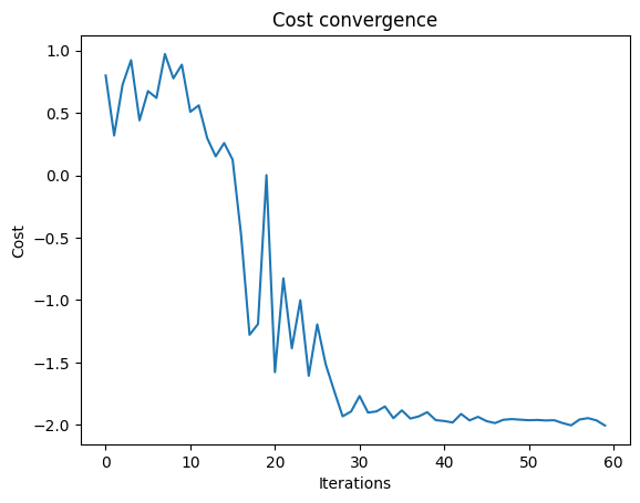
We can check the convergence of the run:
plt.plot(combi.cost_trace)
plt.xlabel("Iterations")
plt.ylabel("Cost")
plt.title("Cost convergence")
Text(0.5, 1.0, 'Cost convergence')
Optimization Results
We can also examine the statistics of the algorithm. The optimization is always defined as a minimzation problem, so the positive maximization objective was tranlated to a negative minimization one by the Pyomo to qmod translator.
In order to get samples with the optimized parameters, we call the sample method:
optimization_result = combi.sample(optimized_params)
optimization_result.sort_values(by="cost").head(5)
| solution | probability | cost | |
|---|---|---|---|
| 3 | {'x': [0, 1, 0, 1, 0, 0, 0, 1]} | 0.098145 | -3 |
| 13 | {'x': [0, 0, 1, 1, 0, 0, 0, 1]} | 0.005371 | -3 |
| 12 | {'x': [1, 1, 0, 1, 0, 0, 0, 0]} | 0.005859 | -3 |
| 0 | {'x': [0, 1, 1, 1, 0, 0, 0, 1]} | 0.319336 | -2 |
| 39 | {'x': [1, 0, 0, 1, 0, 0, 0, 0]} | 0.000977 | -2 |
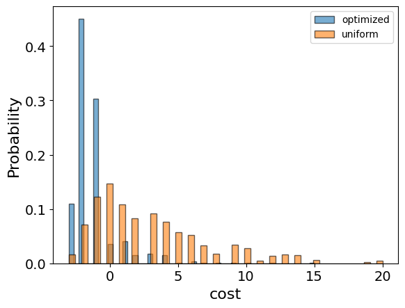
We will also want to compare the optimized results to uniformly sampled results:
uniform_result = combi.sample_uniform()
And compare the histograms:
optimization_result["cost"].plot(
    kind="hist",
    bins=50,
    edgecolor="black",
    weights=optimization_result["probability"],
    alpha=0.6,
    label="optimized",
)
uniform_result["cost"].plot(
    kind="hist",
    bins=50,
    edgecolor="black",
    weights=uniform_result["probability"],
    alpha=0.6,
    label="uniform",
)
plt.legend()
plt.ylabel("Probability", fontsize=16)
plt.xlabel("cost", fontsize=16)
plt.tick_params(axis="both", labelsize=14)
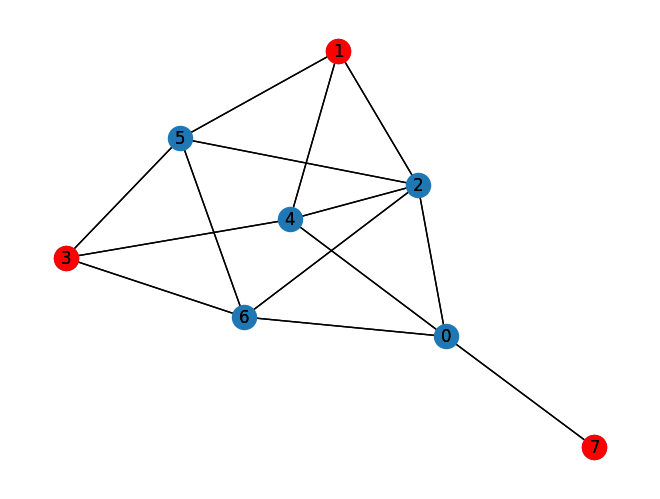
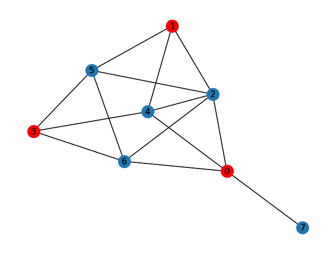
Let us plot the best solution:
best_solution = optimization_result.solution[optimization_result.cost.idxmin()]["x"]
independent_set = [node for node in graph.nodes if best_solution[node] == 1]
print("Independent Set: ", independent_set)
print("Size of Independent Set: ", len(independent_set))
Independent Set:  [1, 3, 7]
Size of Independent Set:  3
nx.draw_kamada_kawai(graph, with_labels=True)
nx.draw_kamada_kawai(
    graph,
    with_labels=True,
    nodelist=independent_set,
    node_color="r",
)
Lastly, we can compare to the classical solution of the problem:
from pyomo.opt import SolverFactory

solver = SolverFactory("couenne")
solver.solve(mis_model)
classical_solution = [pyo.value(mis_model.x[i]) for i in graph.nodes]
independent_set_classical = [
    node for node in graph.nodes if np.allclose(classical_solution[node], 1)
]
print("Classical Independent Set: ", independent_set_classical)
print("Size of Classical Independent Set: ", len(independent_set_classical))
Classical Independent Set:  [0, 1, 3]
Size of Classical Independent Set:  3
nx.draw_kamada_kawai(graph, with_labels=True)
nx.draw_kamada_kawai(
    graph,
    with_labels=True,
    nodelist=independent_set_classical,
    node_color="r",
)
References
[1]: Max Independent Set (Wikipedia)
[2]: Farhi, Edward, Jeffrey Goldstone, and Sam Gutmann. "A quantum approximate optimization algorithm." arXiv preprint arXiv:1411.4028 (2014).
[3]: Barkoutsos, Panagiotis Kl, et al. "Improving variational quantum optimization using CVaR." Quantum 4 (2020): 256.