Deutsch-Jozsa Algorithm
The Deutsch–Jozsa algorithm [1], [2], named after David Deutsch and Richard Jozsa, is one of the first fundamental quantum algorithms showing exponential speedup over its classical counterpart\(^*\). While it has no practical applicative use, it serves as a toy model for quantum computing, demonstrating how the concepts of superposition and interference enable quantum algorithms to outperform classical ones.
The algorithm treats the following problem:
- Input: A black box Boolean function \(f(x)\) that acts on the integers in the range \([0, 2^{n}-1]\).
- Promise: The function is either constant or balanced (for half of the values it is 1 and for the other half it is 0).
- Output: Whether the function is constant or balanced.
Complexity: The quantum approach requires a single query. If we require a deterministic answer to the problem, classically, we must inquire of the oracle \(2^{n-1}+1\) times in the worst case. Therefore, the quantum algorithm exhibits a clear exponential speedup. However, without requiring deterministic determination—namely, allowing application of the classical probabilistic algorithm to get the result up to some error—then the exponential speedup is lost: taking \(k\) classical evaluations of the function \(f\) determines whether the function is constant or balanced, with a probability of \(1 - 1/2^k\).
\(^*\) The exponential speedup is in the oracle complexity setting. It only refers to deterministic classical machines.
Keywords: Foundational quantum algorithms, Phase oracle, Function evaluation, Oracle problem, Oracle/Query complexity.
We define the Deutsch-Jozsa algorithm, which has a quantum part and a classical postprocess part. Then, we run the algorithm on two different examples, one with a simple \(f(x)\) and another that is more complex. A mathematical explanation of the algorithm is provided at the end of this notebook.
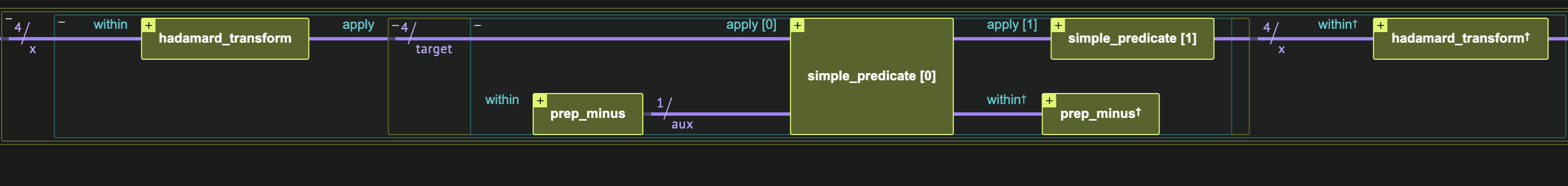
Figure 1. The Deutsch-Jozsa algorithm
How to Build the Algorithm with Classiq
We define a deutsch_jozsa quantum function whose arguments are a quantum function for the black box \(f(x)\), and a quantum variable on which it acts, \(x\). The Deutsch-Jozsa algorithm is composed of three quantum blocks (see Figure 1): a Hadamard transform, an arithmetic oracle for the black box function, and another Hadamard transform.
The Quantum Part
from classiq import *


@qfunc
def deutsch_jozsa(predicate: QCallable[QNum, QBit], x: QNum) -> None:
    within_apply(
        lambda: hadamard_transform(x),
        lambda: phase_oracle(predicate=lambda x, y: predicate(x, y), target=x),
    )
The Classical Postprocess
The classical part of the algorithm reads: The probability of measuring the \(|0\rangle_n\) state is 1 if the function is constant and 0 if it is balanced. We define a classical function that gets the execution results from running the quantum part and returns whether the function is constant or balanced:
def post_process_deutsch_jozsa(parsed_results):
    if len(parsed_results) == 1:
        if 0 not in parsed_results:
            print("The function is balanced")
        else:
            print("The function is constant")
    else:
        print(
            "cannot decide as more than one output was measured, the distribution is:",
            parsed_results,
        )
Example: Simple Arithmetic Oracle
We start with a simple example on \(n=4\) qubits, and \(f(x)= x >7\). Classically, in the worst case, the function should be evaluated \(2^{n-1}+1=9\) times. However, with the Deutsch-Jozsa algorithm, this function is evaluated only once.
We build a predicate for this specific use case:
@qperm
def simple_predicate(x: Const[QNum], res: QBit) -> None:
    res ^= x > 7
Next, we define a model by inserting the predicate into the deutsch_jozsa function:
NUM_QUBITS = 4


@qfunc
def main(x: Output[QNum[NUM_QUBITS]]):
    allocate(x)
    deutsch_jozsa(lambda x, y: simple_predicate(x, y), x)


qprog_1 = synthesize(main)
Finally, we execute and call the classical postprocess:
result_1 = execute(qprog_1).result_value()
results_list_1 = [sample.state["x"] for sample in result_1.parsed_counts]
post_process_deutsch_jozsa(results_list_1)
The function is balanced
show(qprog_1)
Quantum program link: https://platform.classiq.io/circuit/34bVikTQl9GLdAJDoA3darxeyCH
Example: Complex Arithmetic Oracle
Generalizing to more complex scenarios makes no difference for modeling. Let us take a complicated function, working with \(n=3\): a function \(f(x)\) that first takes the maximum between the input bitwise-xor with 4 and the input bitwise-and with 3, then checks whether the result is greater or equal to 4. Can you tell whether the function is balanced or constant?
This time we provide a width bound to the synthesis engine.
We follow the three steps as before:
from classiq.qmod.symbolic import max

NUM_QUBITS = 3


@qperm
def complex_predicate(x: Const[QNum], res: QBit) -> None:
    res ^= max(x ^ 4, x & 3) >= 4


@qfunc
def main(x: Output[QNum[NUM_QUBITS]]):
    allocate(x)
    deutsch_jozsa(lambda x, y: complex_predicate(x, y), x)


qprog_2 = synthesize(
    model=main,
    constraints=Constraints(max_width=19),
)

result_2 = execute(qprog_2).result_value()
results_list_2 = [sample.state["x"] for sample in result_2.parsed_counts]
post_process_deutsch_jozsa(results_list_2)
The function is balanced
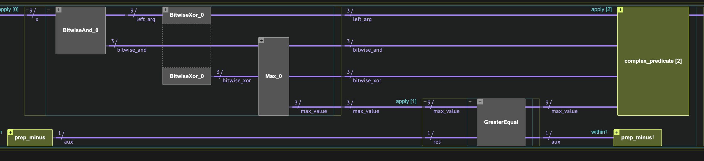
Figure 2. The Deutsch-Jozsa algorithm for the complex example, focusing on oracle implementation (the last block performs uncomputation).
We can visualize the circuit obtained from the synthesis engine. Figure 2 presents the complex structure of the oracle, generated automatically by the synthesis engine.
show(qprog_2)
Quantum program link: https://platform.classiq.io/circuit/34bVjr59eM7JAd2uyXu50Z0iIFt
Technical Notes
A brief summary of the linear algebra behind the Deutsch-Jozsa algorithm. The first Hadamard transformation generates an equal superposition over all the standard basis elements:
The arithmetic oracle gets a Boolean function and adds an \(e^{\pi i}=-1\) phase to all states for which the function returns true:
Finally, applying the Hadamard transform, which can be written as \(H^{\otimes n}\equiv \frac{1}{2^{n/2}}\sum^{2^n-1}_{k,l=0}(-1)^{k\cdot l} |k\rangle \langle l|\), gives
The probability of getting the state \(|k\rangle = |0\rangle\) is
References
-
David Deutsch & Richard Jozsa. Rapid solutions of problems by quantum computation. Proceedings of the Royal Society of London A. 439 (1907): 553–558. (1992).
-
DOI ↗
- Deutsch Jozsa. - (Wikipedia) ↗