Graph Cut Search Problem with Grover Oracle
The "Maximum Cut Problem" (MaxCut) [1] is an example of a combinatorial optimization problem. It refers to finding a partition of a graph into two sets, such that the number of edges between the two sets is the maximum.
Mathematical Formulation
Given a graph \(G=(V,E)\) with \(|V|=n\) nodes and \(E\) edges, a cut is defined as a partition of the graph into two complementary subsets of nodes. In the MaxCut problem we look for a cut where the number of edges between the two subsets is the maximum. We can represent a cut of the graph by a binary vector \(x\) of size \(n\), assigning 0 and 1 to nodes in the first and second subsets, respectively. The number of connecting edges for a given cut is simply given by summing over \(x_i (1-x_j)+x_j (1-x_i)\) for every pair of connected nodes \((i,j)\).
Solving with the Classiq Platform
In this tutorial we define a search problem instead: Given a graph and number of edges, we check if there is a cut in the graph larger than a certain size. We solve the problem using the Grover algorithm.
Defining a Specific Problem Input
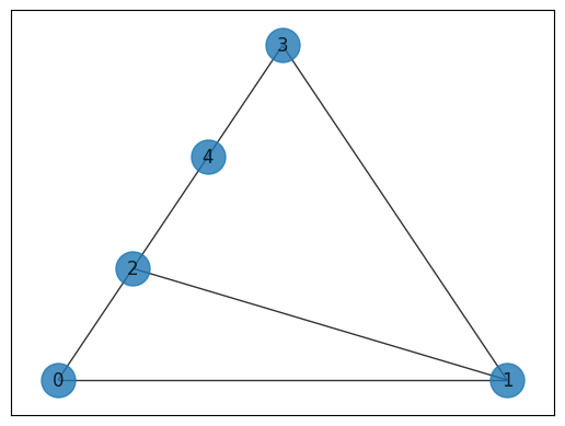
We initiate a specific graph whose maximum cut is 5:
import networkx as nx

# Create graph
G = nx.Graph()
G.add_nodes_from([0, 1, 2, 3, 4])
G.add_edges_from([(0, 1), (0, 2), (1, 2), (1, 3), (2, 4), (3, 4)])
pos = nx.planar_layout(G)
nx.draw_networkx(G, pos=pos, with_labels=True, alpha=0.8, node_size=500)
Creating a Quantum Circuit and Solving It Using the Classiq Platform
We use the grover_search function for the quantum circuit. The oracle function is a phase_oracle, which applies a \((-1)\) phase to each state for which the inner function delivered to phase_oracle returns 1. The cut_oracle is the inner function in this case, calculating whether a given graph partition`s cut is larger than some constant.
Here we look for a cut of size 4 to the graph:
from classiq import *

CUT_SIZE = 4


# cut formulas
def is_cross_cut_edge(x1: int, x2: int) -> int:
    return x1 * (1 - x2) + x2 * (1 - x1)


def cut(x):
    return sum(is_cross_cut_edge(x[node1], x[node2]) for (node1, node2) in G.edges)


# quantum functions
@qfunc
def cut_oracle(cut_size: CInt, nodes: Const[QArray], res: Permutable[QBit]):
    res ^= cut(nodes) >= cut_size


@qfunc
def main(nodes: Output[QArray[QBit, len(G.nodes)]]):
    allocate(nodes)
    grover_search(
        reps=3,
        oracle=lambda vars: phase_oracle(
            lambda vars, res: cut_oracle(CUT_SIZE, vars, res), vars
        ),
        packed_vars=nodes,
    )
Synthesizing the Circuit
We synthesize the circuit using the Classiq synthesis engine. The synthesis takes several seconds:
qmod = create_model(main, constraints=Constraints(max_width=22))
write_qmod(qmod, "grover_max_cut")

qprog = synthesize(qmod)
Showing the Resulting Circuit
After the Classiq synthesis engine finishes the job, we display the resulting circuit in the interactive GUI:
show(qprog)
Quantum program link: https://platform.classiq.io/circuit/2yd4FlAFkOqVH9TVKcHMVWPpDb1
print(qprog.transpiled_circuit.depth)
2666
Executing on a Simulator to Find a Valid Solution
Lastly, we run the resulting circuit on the Classiq execute interface using the execute function.
optimization_result = execute(qprog).result_value()
Upon printing the result, we see that our execution of Grover's algorithm successfully found the satisfying assignments for the input formula:
optimization_result.parsed_counts
[{'nodes': [1, 0, 1, 1, 0]}: 170,
 {'nodes': [1, 0, 0, 0, 1]}: 162,
 {'nodes': [1, 0, 0, 1, 1]}: 161,
 {'nodes': [0, 0, 1, 1, 0]}: 156,
 {'nodes': [1, 0, 0, 1, 0]}: 152,
 {'nodes': [0, 1, 1, 0, 0]}: 151,
 {'nodes': [0, 1, 1, 1, 0]}: 149,
 {'nodes': [1, 1, 0, 0, 1]}: 146,
 {'nodes': [0, 1, 1, 0, 1]}: 136,
 {'nodes': [0, 1, 0, 0, 1]}: 133,
 {'nodes': [1, 0, 1, 0, 0]}: 33,
 {'nodes': [0, 0, 0, 0, 1]}: 31,
 {'nodes': [0, 0, 0, 0, 0]}: 28,
 {'nodes': [1, 1, 0, 1, 0]}: 28,
 {'nodes': [0, 1, 0, 0, 0]}: 27,
 {'nodes': [1, 1, 1, 0, 1]}: 27,
 {'nodes': [0, 1, 1, 1, 1]}: 26,
 {'nodes': [0, 0, 1, 0, 0]}: 25,
 {'nodes': [0, 1, 0, 1, 0]}: 25,
 {'nodes': [1, 1, 1, 1, 0]}: 25,
 {'nodes': [0, 1, 0, 1, 1]}: 24,
 {'nodes': [1, 0, 1, 1, 1]}: 24,
 {'nodes': [0, 0, 1, 1, 1]}: 24,
 {'nodes': [0, 0, 0, 1, 0]}: 23,
 {'nodes': [1, 1, 0, 1, 1]}: 23,
 {'nodes': [0, 0, 0, 1, 1]}: 22,
 {'nodes': [1, 1, 0, 0, 0]}: 21,
 {'nodes': [1, 1, 1, 0, 0]}: 20,
 {'nodes': [1, 0, 0, 0, 0]}: 20,
 {'nodes': [1, 1, 1, 1, 1]}: 19,
 {'nodes': [0, 0, 1, 0, 1]}: 19,
 {'nodes': [1, 0, 1, 0, 1]}: 18]
The satisfying assignments are ~6 times more probable than the unsatisfying assignments. We print one:
most_probable_result = optimization_result.parsed_counts[0]
import matplotlib.pyplot as plt

result_parsed = most_probable_result.state["nodes"]
edge_widths = [
    is_cross_cut_edge(
        int(result_parsed[i]),
        int(result_parsed[j]),
    )
    + 0.5
    for i, j in G.edges
]
node_colors = [int(c) for c in result_parsed]
nx.draw_networkx(
    G,
    pos=pos,
    with_labels=True,
    alpha=0.8,
    node_size=500,
    node_color=node_colors,
    width=edge_widths,
    cmap=plt.cm.rainbow,
)
