Skip to content

Minimum Dominating Set (MDS) Problem

View on GitHub Experiment in the IDE

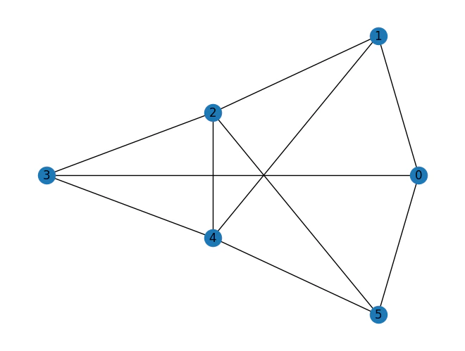
The Minimum Dominating Set problem [1] is a classical NP-hard problem in computer science and graph theory. In this problem, we are given a graph, and we aim to find the smallest subset of vertices such that every node in the graph is either in the subset or is a neighbor of a node in the subset.

We represent the problem as a binary optimization problem.

Variables:

  • \(x_i\) binary variables that represent whether a node \(i\) is in the dominating set or not.

Constraints:

  • Every node \(i\) is either in the dominating set or connected to a node in the dominating set:

\(\forall i \in V: x_i + \sum_{j \in N(i)} x_j \geq 1\)

Where \(N(i)\) represents the neighbors of node \(i\).

Objective

  • Minimize the size of the dominating set:

\(\sum_{i\in V}x_i\)

Solving with the Classiq platform

We go through the steps of solving the problem with the Classiq platform, using QAOA algorithm [2]. The solution is based on defining a pyomo model for the optimization problem we would like to solve.

from typing import cast

import networkx as nx
import numpy as np
import pyomo.core as pyo
from IPython.display import Markdown, display
from matplotlib import pyplot as plt

Building the Pyomo model from a graph input

We proceed by defining the pyomo model that will be used on the Classiq platform, using the mathematical formulation defined above:

import networkx as nx
import pyomo.core as pyo


def mds(graph: nx.Graph) -> pyo.ConcreteModel:
    model = pyo.ConcreteModel()
    model.x = pyo.Var(graph.nodes, domain=pyo.Binary)

    @model.Constraint(graph.nodes)
    def dominating_rule(model, idx):
        sum_of_neighbors = sum(model.x[neighbor] for neighbor in graph.neighbors(idx))
        return model.x[idx] + sum_of_neighbors >= 1

    model.cost = pyo.Objective(expr=sum(model.x.values()), sense=pyo.minimize)

    return model

The model contains:

  • Index set declarations (model.Nodes, model.Arcs).

  • Binary variable declaration for each node (model.x) indicating whether that node is chosen for the set.

  • Constraint rule – for each node, it must be a part of the chosen set or be neighbored by one.

  • Objective rule – the sum of the variables equals the set size.

# generate a random graph
G = nx.erdos_renyi_graph(n=6, p=0.6, seed=8)
nx.draw_kamada_kawai(G, with_labels=True)

mds_model = mds(G)

png

mds_model.pprint()
2 Set Declarations
    dominating_rule_index : Size=1, Index=None, Ordered=False
        Key  : Dimen : Domain : Size : Members
        None :     1 :    Any :    6 : {0, 1, 2, 3, 4, 5}
    x_index : Size=1, Index=None, Ordered=False
        Key  : Dimen : Domain : Size : Members
        None :     1 :    Any :    6 : {0, 1, 2, 3, 4, 5}

1 Var Declarations
    x : Size=6, Index=x_index
        Key : Lower : Value : Upper : Fixed : Stale : Domain
          0 :     0 :  None :     1 : False :  True : Binary
          1 :     0 :  None :     1 : False :  True : Binary
          2 :     0 :  None :     1 : False :  True : Binary
          3 :     0 :  None :     1 : False :  True : Binary
          4 :     0 :  None :     1 : False :  True : Binary
          5 :     0 :  None :     1 : False :  True : Binary

1 Objective Declarations
    cost : Size=1, Index=None, Active=True
        Key  : Active : Sense    : Expression
        None :   True : minimize : x[0] + x[1] + x[2] + x[3] + x[4] + x[5]

1 Constraint Declarations
    dominating_rule : Size=6, Index=dominating_rule_index, Active=True
        Key : Lower : Body                             : Upper : Active
          0 :   1.0 :        x[1] + x[3] + x[5] + x[0] :  +Inf :   True
          1 :   1.0 :        x[0] + x[2] + x[4] + x[1] :  +Inf :   True
          2 :   1.0 : x[1] + x[3] + x[4] + x[5] + x[2] :  +Inf :   True
          3 :   1.0 :        x[0] + x[2] + x[4] + x[3] :  +Inf :   True
          4 :   1.0 : x[1] + x[2] + x[3] + x[5] + x[4] :  +Inf :   True
          5 :   1.0 :        x[0] + x[2] + x[4] + x[5] :  +Inf :   True

5 Declarations: x_index x dominating_rule_index dominating_rule cost

Setting Up the Classiq Problem Instance

In order to solve the Pyomo model defined above, we use the Classiq combinatorial optimization engine. For the quantum part of the QAOA algorithm (QAOAConfig) - define the number of repetitions (num_layers):

from classiq import construct_combinatorial_optimization_model
from classiq.applications.combinatorial_optimization import OptimizerConfig, QAOAConfig

qaoa_config = QAOAConfig(num_layers=6, penalty_energy=8)

For the classical optimization part of the QAOA algorithm we define the maximum number of classical iterations (max_iteration) and the \(\alpha\)-parameter (alpha_cvar) for running CVaR-QAOA, an improved variation of the QAOA algorithm [3]:

optimizer_config = OptimizerConfig(max_iteration=30, alpha_cvar=0.7)

Lastly, we load the model, based on the problem and algorithm parameters, which we can use to solve the problem:

qmod = construct_combinatorial_optimization_model(
    pyo_model=mds_model,
    qaoa_config=qaoa_config,
    optimizer_config=optimizer_config,
)

We also set the quantum backend we want to execute on:

from classiq import set_execution_preferences
from classiq.execution import ClassiqBackendPreferences, ExecutionPreferences

backend_preferences = ExecutionPreferences(
    backend_preferences=ClassiqBackendPreferences(backend_name="simulator")
)

qmod = set_execution_preferences(qmod, backend_preferences)
from classiq import write_qmod

write_qmod(qmod, "minimum_dominating_set")

Synthesizing the QAOA Circuit and Solving the Problem

We can now synthesize and view the QAOA circuit (ansatz) used to solve the optimization problem:

from classiq import show, synthesize

qprog = synthesize(qmod)
show(qprog)
Opening: https://platform.classiq.io/circuit/d5cb21cc-5e64-4e4e-8ea7-414ea1afd2ee?version=0.41.0.dev39%2B79c8fd0855

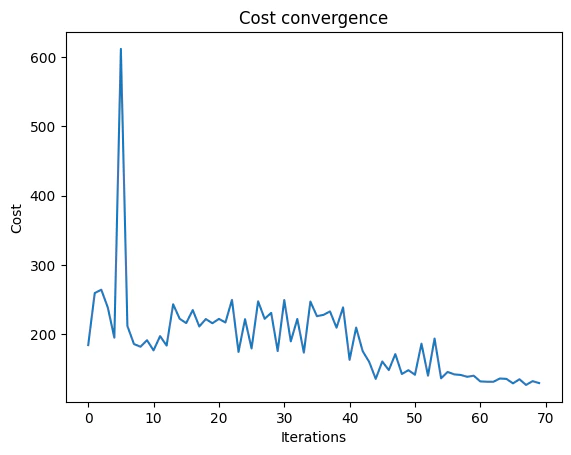
We now solve the problem by calling the execute function on the quantum program we have generated:

from classiq import execute

res = execute(qprog).result()

We can check the convergence of the run:

from classiq.execution import VQESolverResult

vqe_result = res[0].value
vqe_result.convergence_graph

png

Optimization Results

We can also examine the statistics of the algorithm:

import pandas as pd

from classiq.applications.combinatorial_optimization import (
    get_optimization_solution_from_pyo,
)

solution = get_optimization_solution_from_pyo(
    mds_model, vqe_result=vqe_result, penalty_energy=qaoa_config.penalty_energy
)
optimization_result = pd.DataFrame.from_records(solution)
optimization_result.sort_values(by="cost", ascending=True).head(5)
probability cost solution count
707 0.001 2.0 [1, 1, 0, 0, 0, 0] 1
482 0.001 3.0 [0, 0, 1, 1, 0, 1] 1
158 0.001 3.0 [1, 1, 0, 1, 0, 0] 1
121 0.001 4.0 [0, 0, 1, 1, 1, 1] 1
704 0.001 4.0 [1, 0, 0, 1, 1, 1] 1

And the histogram:

optimization_result.hist("cost", weights=optimization_result["probability"])
array([[<Axes: title={'center': 'cost'}>]], dtype=object)

png

Let us plot the solution:

best_solution = optimization_result.solution[optimization_result.cost.idxmin()]
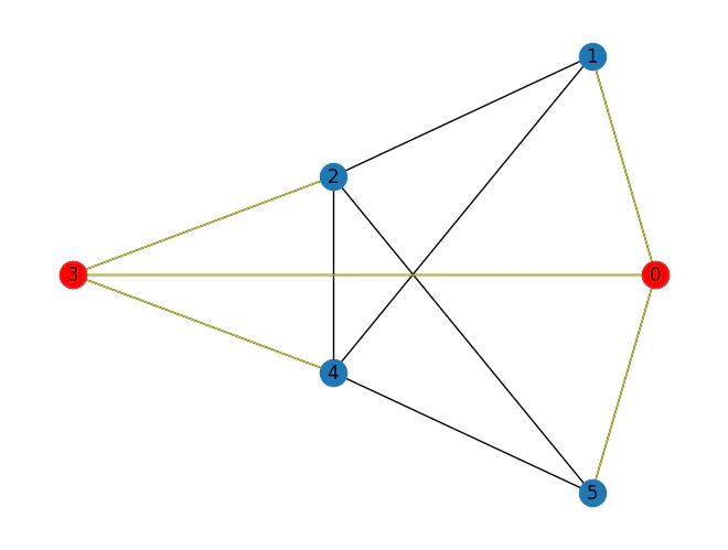
def draw_solution(graph: nx.Graph, solution: list):
    solution_nodes = [v for v in graph.nodes if solution[v]]
    solution_edges = [
        (u, v) for u, v in graph.edges if u in solution_nodes or v in solution_nodes
    ]
    nx.draw_kamada_kawai(graph, with_labels=True)
    nx.draw_kamada_kawai(
        graph,
        nodelist=solution_nodes,
        edgelist=solution_edges,
        node_color="r",
        edge_color="y",
    )


draw_solution(G, best_solution)

png

Lastly, we can compare to the classical solution of the problem:

from pyomo.opt import SolverFactory

solver = SolverFactory("couenne")
solver.solve(mds_model)

mds_model.display()
classical_solution = [int(pyo.value(mds_model.x[i])) for i in G.nodes]
Model unknown

  Variables:
    x : Size=6, Index=x_index
        Key : Lower : Value : Upper : Fixed : Stale : Domain
          0 :     0 :   1.0 :     1 : False : False : Binary
          1 :     0 :   0.0 :     1 : False : False : Binary
          2 :     0 :   0.0 :     1 : False : False : Binary
          3 :     0 :   1.0 :     1 : False : False : Binary
          4 :     0 :   0.0 :     1 : False : False : Binary
          5 :     0 :   0.0 :     1 : False : False : Binary

  Objectives:
    cost : Size=1, Index=None, Active=True
        Key  : Active : Value
        None :   True :   2.0

  Constraints:
    dominating_rule : Size=6
        Key : Lower : Body : Upper
          0 :   1.0 :  2.0 :  None
          1 :   1.0 :  1.0 :  None
          2 :   1.0 :  1.0 :  None
          3 :   1.0 :  2.0 :  None
          4 :   1.0 :  1.0 :  None
          5 :   1.0 :  1.0 :  None
draw_solution(G, classical_solution)

png

References

[1]: Dominating Set (Wikipedia)

[2]: Farhi, Edward, Jeffrey Goldstone, and Sam Gutmann. "A quantum approximate optimization algorithm." arXiv preprint arXiv:1411.4028 (2014).

[3]: Barkoutsos, Panagiotis Kl, et al. "Improving variational quantum optimization using CVaR." Quantum 4 (2020): 256.