Quantum Kernels and Support Vector Machines
Credit card fraud detection - simple use case
QSVM on Kaggle labeled data as means to classify and detect credit card fraudulant transactions
-
Quantum Machine Learning (QML) is the aspect of research that explores the consequences of implementing machine learning on a quantum computer
-
SVM is a supervised machine learning method widely used for multiple labeled data classification.
-
SVM algorithm can be enhanced even on a noisy intermediate scale quantum computer (NISQ) by introducing kernel method.
It can be restructured so that it can exploit the properties of large dimensionality of quantum Hilbert space
-
In this demo we will present a simple use case where Quantum SVM (QSVM) algorithm will be implemented on credit card labeled data to detect fraudulent transactions
-
We will leverage Classiqs proprietary QSVM library and core capabilities to explore the rising potential in enhancing security applications
Demostration is based on recent work published on August 2022 [1]
In this demo, besides the classiq package, we will use the sklearn package
%%capture
! pip install scikit-learn
! pip install seaborn
Importing the required resources:
# General Imports
# Visualisation Imports
import matplotlib.pyplot as plt
import numpy as np
import pandas as pd

# Scikit Imports
import sklearn
from sklearn import datasets
from sklearn.decomposition import PCA
from sklearn.model_selection import train_test_split
from sklearn.preprocessing import MinMaxScaler, StandardScaler
from sklearn.svm import SVC
from sklearn.utils import shuffle
## For TSNE visualisation
from numpy import linalg
from numpy.linalg import norm
from scipy.spatial.distance import pdist, squareform
from sklearn.manifold import TSNE

# We'll hack a bit with the t-SNE code in sklearn 0.15.2.
from sklearn.metrics.pairwise import pairwise_distances
from sklearn.preprocessing import scale

# Random state.
RS = 20150101

import matplotlib
import matplotlib.colors as colors

# We'll use matplotlib for graphics.
import matplotlib.patheffects as PathEffects
import matplotlib.pyplot as plt

# We import seaborn to make nice plots.
try:
    import seaborn as sns
except ModuleNotFoundError:
    palette = np.array(
        [
            (0.4, 0.7607843137254902, 0.6470588235294118),
            (0.9882352941176471, 0.5529411764705883, 0.3843137254901961),
            (0.5529411764705883, 0.6274509803921569, 0.796078431372549),
            (0.9058823529411765, 0.5411764705882353, 0.7647058823529411),
            (0.6509803921568628, 0.8470588235294118, 0.32941176470588235),
            (1.0, 0.8509803921568627, 0.1843137254901961),
            (0.8980392156862745, 0.7686274509803922, 0.5803921568627451),
            (0.7019607843137254, 0.7019607843137254, 0.7019607843137254),
        ]
    )
else:
    sns.set_style("darkgrid")
    sns.set_palette("muted")
    sns.set_context("notebook", font_scale=1.5, rc={"lines.linewidth": 2.5})
    palette = np.array(sns.color_palette("Set2"))

import warnings

warnings.filterwarnings("ignore")
from classiq import *
The Data
The dataset contains transactions made by credit cards in September 2013 by European cardholders.
This dataset presents transactions that occurred in two days, where there were 492 frauds out of 284,807 transactions. The dataset is highly unbalanced, the positive class (frauds) account for 0.172% of all transactions.
Data properties:
-
Database contains only numeric input variables which are the result of a PCA transformation.
-
Due to confidentiality issues, original features are not provided.
-
Features V1, V2, … V28 are the principal components obtained with PCA.
-
The only features which have not been transformed with PCA are 'Time' and 'Amount'.
-
Feature 'Time' contains the seconds elapsed between each transaction and the first transaction in the dataset.
-
The feature 'Amount' is the transaction Amount.
-
Feature 'Class' is the response variable and it takes value 1 in case of fraud and 0 otherwise.
Data is freely available through Kaggle [2]
Loading the Kaggle "Credit Card Fraud Detection" data set
import pathlib

path = (
    pathlib.Path(__file__).parent.resolve()
    if "__file__" in locals()
    else pathlib.Path(".")
)
input_file = path / "../resources/creditcard.csv"
# comma delimited file as input
kaggle_full_set = pd.read_csv(input_file, header=0)
# presnting first 5 lines:
kaggle_full_set.head()
| Time | V1 | V2 | V3 | V4 | V5 | V6 | V7 | V8 | V9 | ... | V21 | V22 | V23 | V24 | V25 | V26 | V27 | V28 | Amount | Class | |
|---|---|---|---|---|---|---|---|---|---|---|---|---|---|---|---|---|---|---|---|---|---|
| 0 | 0 | -1.359807 | -0.072781 | 2.536347 | 1.378155 | -0.338321 | 0.462388 | 0.239599 | 0.098698 | 0.363787 | ... | -0.018307 | 0.277838 | -0.110474 | 0.066928 | 0.128539 | -0.189115 | 0.133558 | -0.021053 | 149.62 | 0 |
| 1 | 0 | 1.191857 | 0.266151 | 0.166480 | 0.448154 | 0.060018 | -0.082361 | -0.078803 | 0.085102 | -0.255425 | ... | -0.225775 | -0.638672 | 0.101288 | -0.339846 | 0.167170 | 0.125895 | -0.008983 | 0.014724 | 2.69 | 0 |
| 2 | 1 | -1.358354 | -1.340163 | 1.773209 | 0.379780 | -0.503198 | 1.800499 | 0.791461 | 0.247676 | -1.514654 | ... | 0.247998 | 0.771679 | 0.909412 | -0.689281 | -0.327642 | -0.139097 | -0.055353 | -0.059752 | 378.66 | 0 |
| 3 | 1 | -0.966272 | -0.185226 | 1.792993 | -0.863291 | -0.010309 | 1.247203 | 0.237609 | 0.377436 | -1.387024 | ... | -0.108300 | 0.005274 | -0.190321 | -1.175575 | 0.647376 | -0.221929 | 0.062723 | 0.061458 | 123.50 | 0 |
| 4 | 2 | -1.158233 | 0.877737 | 1.548718 | 0.403034 | -0.407193 | 0.095921 | 0.592941 | -0.270533 | 0.817739 | ... | -0.009431 | 0.798278 | -0.137458 | 0.141267 | -0.206010 | 0.502292 | 0.219422 | 0.215153 | 69.99 | 0 |
5 rows × 31 columns
Selecting training and testing data sets
To proceed with the analysis, we sub-sample the dataset to make it manageable for near-term quantum simulations
TRAIN_NOMINAL_SIZE = 100
TRAIN_FRAUD_SIZE = 25

TEST_NOMINAL_SIZE = 50
TEST_FRAUD_SIZE = 10

PREDICTION_NOMINAL_SIZE = 50
PREDICTION_FRAUD_SIZE = 10

SHUFFLE_DATA = False
## Seperating nominal ("legit") from fraud:
all_fraud_set = kaggle_full_set.loc[kaggle_full_set["Class"] == 1]
all_nominal_set = kaggle_full_set.loc[kaggle_full_set["Class"] == 0]
## Optionally shuffle data before selctive sets
if SHUFFLE_DATA:
    all_fraud_set = shuffle(all_fraud_set, random_state=1234)
    all_nominal_set = shuffle(all_nominal_set, random_state=1234)
## Selecting data subsets
selected_training_set = pd.concat(
    [all_nominal_set[:TRAIN_NOMINAL_SIZE], all_fraud_set[:TRAIN_FRAUD_SIZE]]
)
selected_testing_set = pd.concat(
    [
        all_nominal_set[TRAIN_NOMINAL_SIZE : TRAIN_NOMINAL_SIZE + TEST_NOMINAL_SIZE],
        all_fraud_set[TRAIN_FRAUD_SIZE : TRAIN_FRAUD_SIZE + TEST_FRAUD_SIZE],
    ]
)
selected_prediction_set = pd.concat(
    [
        all_nominal_set[
            TRAIN_NOMINAL_SIZE
            + TEST_NOMINAL_SIZE : TRAIN_NOMINAL_SIZE
            + TEST_NOMINAL_SIZE
            + PREDICTION_NOMINAL_SIZE
        ],
        all_fraud_set[
            TRAIN_FRAUD_SIZE
            + TEST_FRAUD_SIZE : TRAIN_FRAUD_SIZE
            + TEST_FRAUD_SIZE
            + PREDICTION_FRAUD_SIZE
        ],
    ]
)
## Seperating relevant features data (excluding the "Time" colom) from label data

kaggle_headers = list(kaggle_full_set.columns.values)  # all headers
feature_cols = kaggle_headers[1:-1]  # excluding Time and Class headers
label_col = kaggle_headers[-1]  # marking Class header as label

selected_training_data = selected_training_set.loc[:, feature_cols]
selected_training_labels = selected_training_set.loc[:, label_col]

selected_testing_data = selected_testing_set.loc[:, feature_cols]
selected_testing_labels = selected_testing_set.loc[:, label_col]

selected_prediction_data = selected_prediction_set.loc[:, feature_cols]
selected_prediction_true_labels = selected_prediction_set.loc[:, label_col]
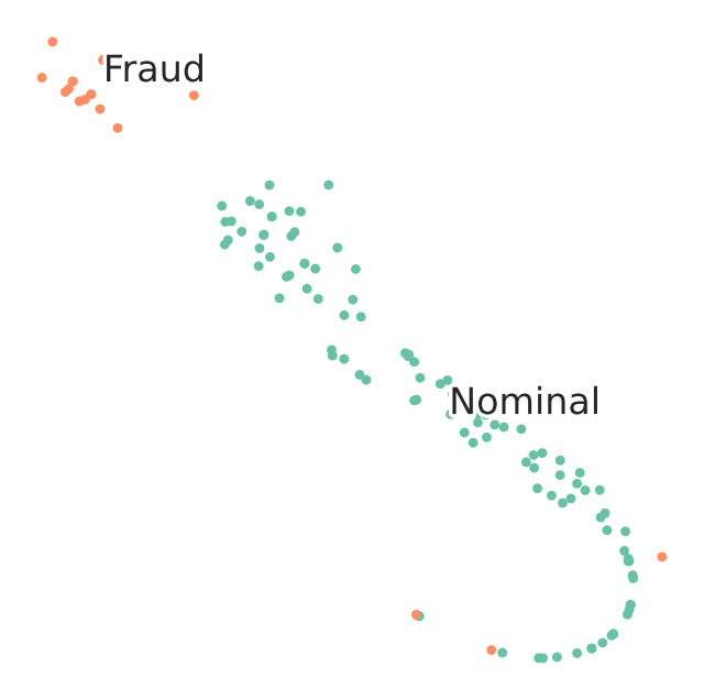
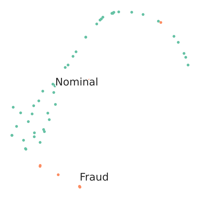
Visualization of the selected data sets with t-SNE
t-SNE is a technique for dimensionality reduction that is particularly suited for the visualization of high-dimensional datasets
def scatter(x, colors):
    # We create a scatter plot.
    f = plt.figure(figsize=(8, 8))
    ax = plt.subplot(aspect="equal")
    sc = ax.scatter(x[:, 0], x[:, 1], lw=0, s=40, c=palette[colors.astype(np.int32)])
    plt.xlim(-25, 25)
    plt.ylim(-25, 25)
    ax.axis("off")
    ax.axis("tight")

    # We add the labels for each digit.
    txts = []
    labels = ["Nominal", "Fraud"]
    for i in range(2):
        # Position of each label.
        xtext, ytext = np.median(x[colors == i, :], axis=0)
        txt = ax.text(xtext, ytext, labels[i], fontsize=24)
        txt.set_path_effects(
            [PathEffects.Stroke(linewidth=5, foreground="w"), PathEffects.Normal()]
        )
        txts.append(txt)

    return
TSNE Visualization of train data
We observe that visually t-SNE shows a separation between nominal and anomalous samples.
However, sole visualization map does not allow to track all fraudulent transactions.
This demonstrates the challenge of high-quality fraud detection.
For the sake of quick demonstration we subselcetd a very small percentage of the data. Better logic for sub selecting the training and testing datasets will effect quality of results.
proj = TSNE(random_state=RS).fit_transform(selected_training_data)
scatter(proj, selected_training_labels)
TSNE Visualization of test data
proj = TSNE(random_state=RS).fit_transform(selected_testing_data)
scatter(proj, selected_testing_labels)
Reduce dimensions
Convert original features into fewer features to match the number of Qubits
We perform dimensionality reduction to match the number of features with the number of qubits used in simulation. For this, we use principal component analysis and keep only the first N_DIM principal components.
## choosing data dimension to encode
N_DIM = 3
sample_train = selected_training_data.values.tolist()
sample_test = selected_testing_data.values.tolist()
sample_predict = selected_prediction_data.values.tolist()

# Reduce dimensions

pca = PCA(n_components=N_DIM).fit(sample_train)
sample_train = pca.transform(sample_train)
sample_test = pca.transform(sample_test)
sample_predict = pca.transform(sample_predict)
Normalize
We use feature-wise standard scaling, i.e. we subtract the mean and scale by the standard deviation for each feature
# Normalize
std_scale = StandardScaler().fit(sample_train)
sample_train = std_scale.transform(sample_train)
sample_test = std_scale.transform(sample_test)
sample_predict = std_scale.transform(sample_predict)
Scale
Scaling each feature to a range between -\(\pi\) and \(\pi\).
# Scale
samples = np.append(sample_train, sample_test, axis=0)
samples = np.append(samples, sample_predict, axis=0)
minmax_scale = MinMaxScaler((-np.pi, np.pi)).fit(samples)
FRAUD_TRAIN_DATA = minmax_scale.transform(sample_train)
FRAUD_TEST_DATA = minmax_scale.transform(sample_test)
FRAUD_PREDICT_DATA = minmax_scale.transform(sample_predict)
Final preprocessed data set
FRAUD_TRAIN_LABELS = np.array(selected_training_labels.values.tolist())
FRAUD_TEST_LABELS = np.array(selected_testing_labels.values.tolist())
FeatureMap design with Classiq
The feature map is a parameterized quantum circuit, which can be described as a unitary transformation \(\mathbf{U_\phi}(\mathbf{x})\) on n qubits.
Since the data may be non-linearly-separable in the original space, the feature map circuit will map the classical data into Hilbert space.
The choice of which feature map circuit to use is key and may depend on the given dataset we want to classify. We will leverage Classiq feature map design capabilities
Build a feature map
As an example we can choose from the well known the Second-order Pauli-Z evolution encoding circuit with 2 repetitions or the bloch sphere circuit encoding. The definition of those are given in tutorials 1 and 2.
The Pauli feature map
from itertools import combinations

import numpy as np


def generate_connectivity_map(list_size, sublist_size, connectivity_type):
    """
    Generate connectivity for a given list size and sublist size.

    Parameters:
    - list_size: The size of the list (number of elements).
    - sublist_size: The size of the subsets to generate.
    - connectivity_type: an integer (0 for linear, 1 for circular, 2 for full)

    Returns:
    - A list of all unique subsets of the given size.
    """
    assert connectivity_type in [
        0,
        1,
        2,
    ], "connectivity must be 0 (linear), 1 (circular), or 2 (full)"

    if connectivity_type == 0:  # linear
        return [
            list(range(i, i + sublist_size))
            for i in range(list_size - sublist_size + 1)
        ]

    elif connectivity_type == 1:  # circular
        return [
            [(i + j) % list_size for j in range(sublist_size)] for i in range(list_size)
        ]

    elif connectivity_type == 2:  # full
        return [list(comb) for comb in combinations(range(list_size), sublist_size)]


def generate_hamiltonian(
    data: CArray[CReal],
    paulis_list: list[list[Pauli]],
    affines: list[list[float]],
    connectivity: int,
) -> tuple[list[list[Pauli]], list[CReal]]:
    assert connectivity in [
        0,
        1,
        2,
    ], "connectivity must be 0 (linear), 1 (circular) or 2 (full)"
    res_paulis = []
    res_coefficients = []
    ham0 = [Pauli.I] * data.len
    for paulis, affine in zip(paulis_list, affines):
        indices = generate_connectivity_map(data.len, paulis.len, connectivity)
        for k in range(len(indices)):
            ham_temp = ham0.copy()
            coe_temp = 1
            for j in range(len(indices[0])):
                ham_temp[indices[k][j]] = paulis[j]
                coe_temp *= affine[0] * (data[indices[k][j]] - affine[1])
            res_paulis.append(ham_temp)
            res_coefficients.append(coe_temp)
    return res_paulis, res_coefficients


@qfunc
def pauli_kernel(
    data: CArray[CReal],
    paulis_list: list[list[Pauli]],
    affines: list[list[float]],
    connectivity: int,
    reps: CInt,
    qba: QArray[QBit],
) -> None:
    paulis, coefficients = generate_hamiltonian(
        data, paulis_list, affines, connectivity
    )
    power(
        reps,
        lambda: (
            hadamard_transform(qba),
            parametric_suzuki_trotter(
                paulis=paulis,
                coefficients=coefficients,
                evolution_coefficient=-1,
                order=1,
                repetitions=1,
                qbv=qba,
            ),
        ),
    )
The Bloch sphere feature map
from classiq.qmod.symbolic import ceiling, floor


@qfunc
def bloch_feature_map(data: CArray[CReal], qba: QArray[QBit]):
    repeat(ceiling(data.len / 2), lambda i: RX(data[2 * i] / 2, qba[i]))
    repeat(floor(data.len / 2), lambda i: RZ(data[(2 * i) + 1], qba[i]))
Finally, we constuct the quantum model for the QSVM routine:
## Choosing "bloch sphere" feature map encoding:


@qfunc
def main(
    data1: CArray[CReal, N_DIM],
    data2: CArray[CReal, N_DIM],
    qba: Output[QNum],
):

    allocate(ceiling(data1.len / 2), qba)
    bloch_feature_map(data1, qba)
    invert(lambda: bloch_feature_map(data2, qba))


QSVM_FRAUD_BLOCH_SHPERE = create_model(main)

## Choosing "Pauli ZZ" feature map encodign with 2 repetitions:
PAULIS = [[Pauli.Z], [Pauli.Z, Pauli.Z]]
CONNECTIVITY = 2  # Full
AFFINES = [[1, 0], [1, np.pi]]
REPS = 2


@qfunc
def main(data1: CArray[CReal, N_DIM], data2: CArray[CReal, N_DIM], qba: Output[QNum]):
    allocate(data1.len, qba)
    pauli_kernel(data1, PAULIS, AFFINES, CONNECTIVITY, REPS, qba)
    invert(lambda: pauli_kernel(data2, PAULIS, AFFINES, CONNECTIVITY, REPS, qba))


QSVM_FRAUD_PAULI_ZZ = create_model(main)
write_qmod(QSVM_FRAUD_PAULI_ZZ, "credit_card_fraud", symbolic_only=False)
Synthesize our model and explore the generated quantum circuit
Once we constructed our qsvm model - we synthesize and view the quantum circuit that encodes our data.
For this we will use classiq built-in synthesize and show functions:
qprog = synthesize(QSVM_FRAUD_PAULI_ZZ)
show(qprog)
Opening: https://platform.classiq.io/circuit/2rMbAbTtY6MnwYp7Jiarxu1yXvF?version=0.65.1
Quantum Support Vector Machines is the Quantum version of SVM - a data classification method which separates the data using a hyperplane.
The algorithm will perform the following steps [3]:
-
Estimating the kernel matrix
-
A quantum feature map, \(\phi(\mathbf{x})\), naturally gives rise to a quantum kernel, \(k(\mathbf{x}_i,\mathbf{x}_j)= \phi(\mathbf{x}_j)^\dagger\phi(\mathbf{x}_i)\), which can be seen as a measure of similarity: \(k(\mathbf{x}_i,\mathbf{x}_j)\) is large when \(\mathbf{x}_i\) and \(\mathbf{x}_j\) are close.
-
When considering finite data, we can represent the quantum kernel as a matrix: \(K_{ij} = \left| \langle \phi^\dagger(\mathbf{x}_j)| \phi(\mathbf{x}_i) \rangle \right|^{2}\).
We can calculate each element of this kernel matrix on a quantum computer by calculating the transition amplitude:
-
This provides us with an estimate of the quantum kernel matrix, which will be used in the support vector classification.
- Optimizing the dual problem by using the classical SVM algorithm to generate a separating Hyperplane and classify the data
- Where $t$ is the amount of data points

- the $\vec{x}_i$s are the data points

- $y_i$ is the label $\in \{-1,1\}$ of each data point

- $K(\vec{x}_i \vec{x}_j)$ is the kernel matrix element between the $i$ and $j$ datapoints

- We optimize over the $\alpha$s

- We expect most of the $\alpha$s to be $0$. The $\vec{x}_i$s that correspond to non-zero $\alpha_i$ are called the Support Vectors.
Setup Classiq QSVM post-process routine:
def get_execution_params(data1, data2=None):
    """
    Generate execution parameters based on the mode (train or validate).

    Parameters:
    - data1: First dataset (used for both training and validation).
    - data2: Second dataset (only required for validation).

    Returns:
    - A list of dictionaries with execution parameters.
    """
    if data2 is None:
        # Training mode (symmetric pairs of data1)
        return [
            {"data1": data1[k], "data2": data1[j]}
            for k in range(len(data1))
            for j in range(k, len(data1))  # Avoid symmetric pairs
        ]
    else:
        # Prediction mode
        return [
            {"data1": data1[k], "data2": data2[j]}
            for k in range(len(data1))
            for j in range(len(data2))
        ]


def construct_kernel_matrix(matrix_size, res_batch, train=False):
    """
    Construct a kernel matrix from `res_batch`, depending on whether it's for training or predicting.

    Parameters:
    - matrix_size: Tuple of (number of rows, number of columns) for the matrix.
    - res_batch: Precomputed batch results.
    - train: Boolean flag. If True, assumes training (symmetric matrix).

    Returns:
    - A kernel matrix as a NumPy array.
    """
    rows, cols = matrix_size
    kernel_matrix = np.zeros((rows, cols))

    num_shots = res_batch[0].num_shots
    num_output_qubits = len(next(iter(res_batch[0].counts)))

    count = 0
    if train:  # and rows == cols:
        # Symmetric matrix (training)
        for k in range(rows):
            for j in range(k, cols):
                value = (
                    res_batch[count].counts.get("0" * num_output_qubits, 0) / num_shots
                )
                kernel_matrix[k, j] = value
                kernel_matrix[j, k] = value  # Use symmetry
                count += 1
    else:
        # Non-symmetric matrix (validation)
        for k in range(rows):
            for j in range(cols):
                kernel_matrix[k, j] = (
                    res_batch[count].counts.get("0" * num_output_qubits, 0) / num_shots
                )
                count += 1

    return kernel_matrix


def train_svm(es, train_data, train_labels):
    """
    Trains an SVM model using a custom precomputed kernel from the training data.

    Parameters:
    - es: ExecutionSession object to process batch execution for kernel computation.
    - train_data: List of data points for training.
    - train_labels: List of binary labels corresponding to the training data.

    Returns:
    - svm_model: A trained SVM model using the precomputed kernel.
    """
    train_size = len(train_data)
    train_execution_params = get_execution_params(train_data)
    res_train_batch = es.batch_sample(train_execution_params)  # execute batch
    # generate kernel matrix for train
    kernel_train = construct_kernel_matrix(
        matrix_size=(train_size, train_size), res_batch=res_train_batch, train=True
    )
    svm_model = SVC(kernel="precomputed")
    svm_model.fit(
        kernel_train, train_labels
    )  # the fit gets the precomputed matrix of training, and the training labels

    return svm_model


def predict_svm(es, data, train_data, svm_model):
    """
    Predicts labels for new data using a precomputed kernel with a trained SVM model.

    Parameters:
    - es: ExecutionSession object to process batch execution for kernel computation.
    - data (list): List of new data points to predict.
    - train_data (list): Original training data used to train the SVM.
    - svm_model: A trained SVM model returned by `train_svm`.

    Returns:
    - y_predict (list): Predicted labels for the input data.
    """
    predict_size = len(data)
    train_size = len(train_data)
    predict_execution_params = get_execution_params(data, train_data)
    res_predict_batch = es.batch_sample(predict_execution_params)  # execute batch
    kernel_predict = construct_kernel_matrix(
        matrix_size=(predict_size, train_size), res_batch=res_predict_batch, train=False
    )
    y_predict = svm_model.predict(
        kernel_predict
    )  # the predict gets the precomputed test matrix

    return y_predict
Run QSVM and analyze results
Train and test the data
-
Build the train and test quantum kernel matrices.
-
For each pair of datapoints in the training dataset \(\mathbf{x}_{i},\mathbf{x}_j\), apply the feature map and measure the transition probability}: \(K_{ij} = \left| \langle 0 | \mathbf{U}^\dagger_{\Phi(\mathbf{x_j})} \mathbf{U}_{\Phi(\mathbf{x_i})} | 0 \rangle \right|^2\).
-
For each training datapoint \(\mathbf{x_i}\) and testing point \(\mathbf{y_i}\), apply the feature map and measure the transition probability: \(K_{ij} = \left| \langle 0 | \mathbf{U}^\dagger_{\Phi(\mathbf{y_i})} \mathbf{U}_{\Phi(\mathbf{x_i})} | 0 \rangle \right|^2\).
-
-
Use the train and test quantum kernel matrices in a classical support vector machine classification algorithm.
Executing QSVM is done though the batch_sample of the ExecutionSession object, as defined in the classical post-process functions above. We consider the accuracy of the classification and the predicted labels for the predict data.
from classiq.execution import ExecutionSession

with ExecutionSession(qprog) as es:
    # train
    svm_model = train_svm(es, FRAUD_TRAIN_DATA.tolist(), FRAUD_TRAIN_LABELS.tolist())

    # test
    y_test = predict_svm(
        es, FRAUD_TEST_DATA.tolist(), FRAUD_TRAIN_DATA.tolist(), svm_model
    )
    test_score = sum(y_test == FRAUD_TEST_LABELS.tolist()) / len(
        FRAUD_TEST_LABELS.tolist()
    )

    # predict
    predicted_labels = predict_svm(
        es, FRAUD_PREDICT_DATA.tolist(), FRAUD_TRAIN_DATA.tolist(), svm_model
    )
print("quantum kernel classification test score: %0.2f" % (test_score))
quantum kernel classification test score: 0.92
Result seems quite good. It's a good start! Let's analyze it further:
Compare testing accuracy results to classical kernels:
classical_kernels = ["linear", "poly", "rbf", "sigmoid"]

for ckernel in classical_kernels:
    classical_svc = SVC(kernel=ckernel)
    classical_svc.fit(FRAUD_TRAIN_DATA, FRAUD_TRAIN_LABELS)
    classical_score = classical_svc.score(
        FRAUD_TEST_DATA, np.array(FRAUD_TEST_LABELS.tolist())
    )

    print("%s kernel classification test score:  %0.2f" % (ckernel, classical_score))
linear kernel classification test score:  1.00
poly kernel classification test score:  1.00
rbf kernel classification test score:  1.00
sigmoid kernel classification test score:  0.98
Given our simple naive training and testing set example, the Quantum kernel gets results "at least as good as" the classical kernels - can be interpetted as prominsing sign and encourage deeper research. Baring in mind the following:
-
Quantum kernel machine algorithms only have the potential of quantum advantage over classical approaches if the corresponding quantum kernel is hard to estimate classically (a necessary and not always sufficient condition to obtain a quantum advantage)
-
However, it was proven recently [4] that learning problems exist for which learners with access to quantum kernel methods have a quantum advantage over all classical learners.
Predict data
Finally, we may predict unlabeled data by calculating the kernel matrix of the new datum with respect to the support vectors
    - Where $\vec{s}$ is the datapoint to be classified

    - $\alpha_i^*$ are the optimized $\alpha$s

    - And $b$ is the bias.
true_labels = np.array(selected_prediction_true_labels.values.tolist())
sklearn.metrics.accuracy_score(predicted_labels, true_labels)
0.9333333333333333
References
[1]: Oleksandr Kyriienko, Einar B. Magnusson "Unsupervised quantum machine learning for fraud detection"
[2]: Kaggle dataset - Credit Card Fraud Detection Anonymized credit card transactions labeled as fraudulent or genuine
[3]: Havlíček, V., Córcoles, A.D., Temme, K. et al. Supervised learning with quantum-enhanced feature spaces. Nature 567, 209-212 (2019)
[4]: Liu et al. A rigorous and robust quantum speed-up in supervised machine learning (2020)