Execute
The last step of the quantum algorithm development process with Classiq is to execute the quantum program on a quantum computer or a simulator. This can be done in the IDE or through the Python SDK. Classiq offers access to a wide variety of quantum computers with different hardware modalities from several companies including: IonQ, Quantinuum, IBM, OQC and Rigetti, as well as to several simulators.
The execution phase is composed of configuration and access to the results. In the following, we cover these parts through a concrete example. First we start with the default execution options of Classiq, the execution we have encountered in previous example of this 101 guide.
Default Execution
Continuing with the algorithm from previous chapters, we want to create a quantum algorithm that calculates in a superposition the arithmetic expression \(y=x^2+1\). The following algorithm written in Qmod implements the desired task:
from classiq import *


@qfunc
def main(x: Output[QNum], y: Output[QNum]):

    allocate(4, x)
    hadamard_transform(x)  # creates a uniform superposition
    y |= x**2 + 1
qfunc main(output x: qnum, output y: qnum) {
  allocate<4>(x);
  hadamard_transform(x);
  y = (x ** 2) + 1;
}
And the algorithm can then be synthesized:
quantum_program = synthesize(create_model(main))
The quantum program at hand can now be executed directly and the results can be analyzed:
job = execute(quantum_program)
results = job.result()[0].value.parsed_counts
print(results)
The above demonstrates how the execution can be done with the default configuration of Classiq which is an execution on a simulator (with up to 25 qubits) with 1000 shots. Let's see how we can execute with other configurations.
Configuring the Execution
Configuration in the IDE
From the IDE, the execution configuration is done via the Execution tab, which is automatically accesses when the Execute button is pressed from the visualization of the quantum program:
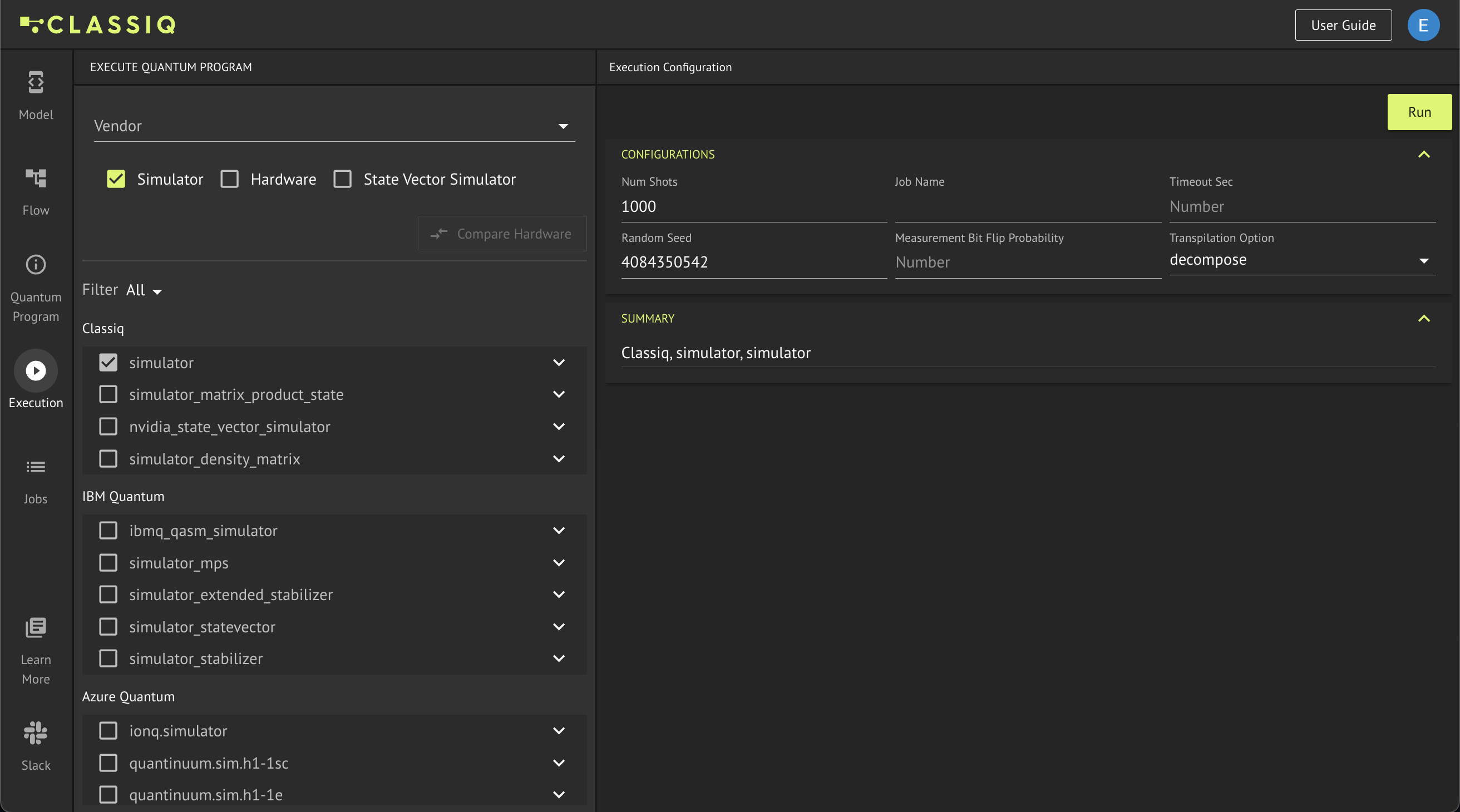
On the left-hand side one can see a list of all the available simulators that can be accessed. On the top part, one can tick the Hardware box to see a lost of all the available hardwares one can access via the platform. The hardwares as well as some of the simulators require further credentials that needs to be entered once the Run button is pressed. These credentials are the vendor's credentials for accessing the relevant compute resources (more details can be found in the reference manual).
On the right-hand side of the screen, one can configure the specific execution. The Num Shots can be used to change the number of shots the quantum program will be sampled, and one can enter an indicative Job Name. The Random Seed can be used in order to receive the exact same results when a simulator is used (as well as for more advanced execution options on real hardware such as variational quantum algorithms and advanced transpilation methods).
After the configuration is done, all that remains is to press to Run button.
Configuration in the SDK
One can change the execution configuration from the SDK as well. This is done by adapting the quantum model with the desired execution preferences, similarly to the constraints and preferences from the optimization phase.
The following code demonstrates how to change the number of shots, to set a name for the job and to set a random seed for the simulator:
from classiq.execution import ExecutionPreferences

quantum_model = create_model(main)
quantum_model_with_execution_preferences = set_execution_preferences(
    quantum_model,
    ExecutionPreferences(
        num_shots=2048, job_name="classiq 101 - execute", random_seed=767
    ),
)
And then the adapted quantum model can be synthesized and executed:
quantum_program_with_execution_preferences = synthesize(
    quantum_model_with_execution_preferences
)
job = execute(quantum_program_with_execution_preferences)
The full list of configuration options for the execution preferences can be found in the reference manual.
Accessing the Results
Results in the IDE
Once you press the Run button from the Execution tab you will automatically be transitioned to the Jobs tab of the platform. All your jobs are listed on the left-hand side, and by clicking on a specific job, its information is depicted below the job name.
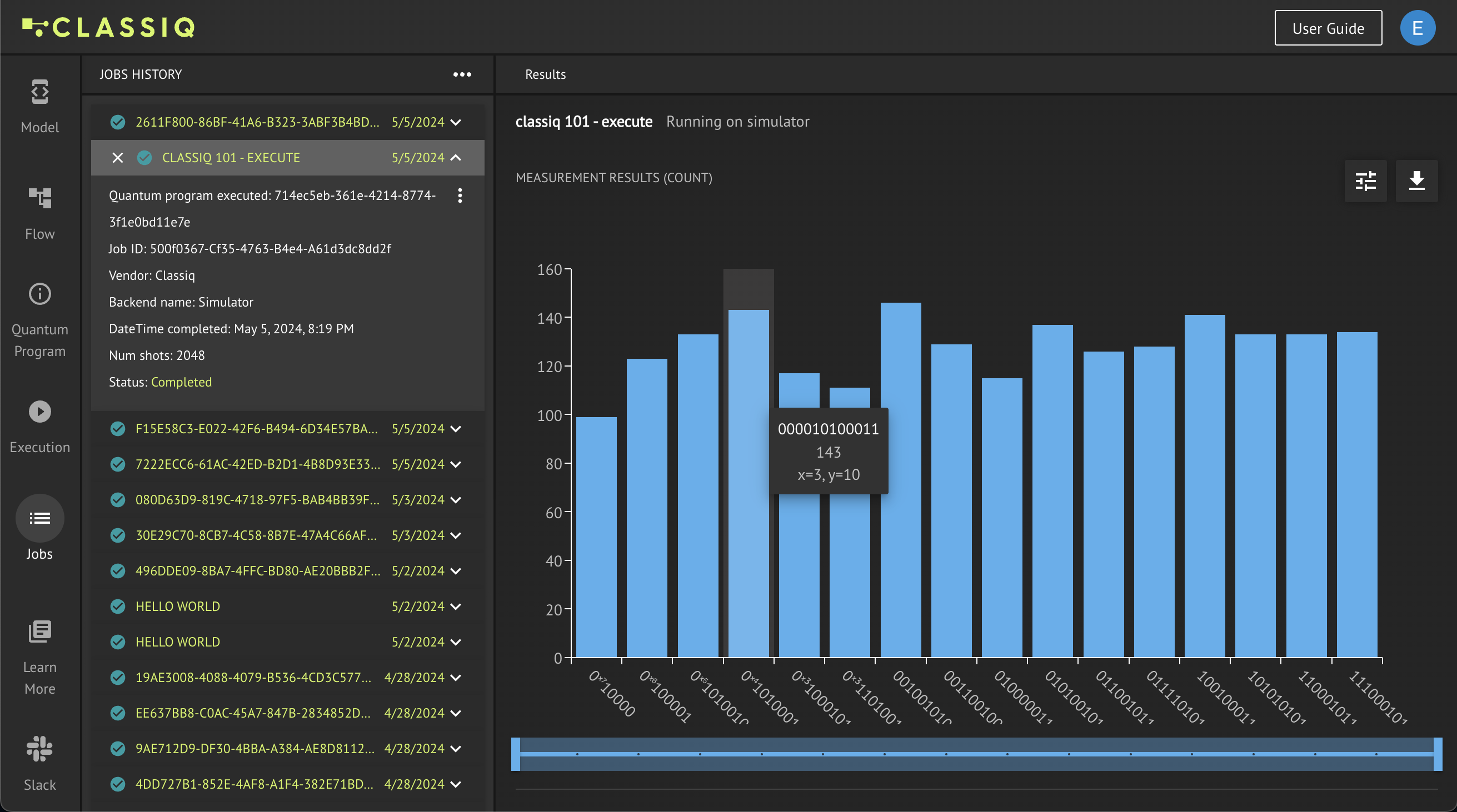
On the right-hand side, the histogram of the results is depicted. Each bin represent a specific measurement result and its hight represents the counts of that measurement. By hovering over a specific bin, the variables of that measurement results are depicted, as well as the counts of that bin.
At the top-right corner there are two buttons. The right one allows downloading the results of the job in a specific format like .csv, and the left button enables further options for analyzing the histogram results.
Results in the SDK
The job variable which is the output of the execute command contains all the data about the execution job. Some of the meta data can be accessed directly from this object:
print(
    f"The job on the provider {job.provider} on the backend {job.backend_name} with {job.num_shots} shots is {job.status} can be accessed in the IDE with this URL: {job.ide_url}"
)
In addition to the meta data, we see the option to open the job also in the IDE. This can be done directly with:
job.open_in_ide()
The actual results of the job can be accessed with:
results = job.result()[0].value
The results variable contains a dictionary of the measured variables of our algorithm and their respective counts:
print(results.parsed_counts)
The raw bit strings can also be accessed directly with:
print(results.counts)
And the direct mapping between the bit strings and the measured variables can aldo be extracted:
print(results.parsed_states)
The notation of wether the bit strings are interpreted with the least significant bit (LSB) on the right or on the left can also be extracted:
print(results.counts_lsb_right)
All the above should enable one to analyze the results and post-process them in Python as needed.
Verify Your Understanding - Recommended Exercise
Adapt the code such that the quantum number \(x\) is allocated with 8 qubits. Then, execute the algorithm with 5096 shots and post process the results from your Python SDK. Plot a graph of all the measured values of \(x\) and \(y\) with the corresponding axes (make sure you receive the graph of \(y=x^2+1\)).
write_qmod(quantum_model_with_execution_preferences, "execute")