Phase Kickback
Phase kickback [1,2,3] is an important and highly used primitive in quantum computing. The algorithm deals with "kicking" the result of a function to the phase of a quantum state so it can be wisely manipulated with interferences to achieve the desired result. Every quantum algorithm can be decomposed into these steps: 1) Encoding the data, 2) Manipulating the data, and 3) Extracting the result. The phase kickback primitive is a key step in manipulating the data, enabling the extraction of the result. See the Deutsch-Jozsa and Simon's algorithms for concrete examples.
The standard way [4] of applying a classical function \(f:\{0,1\}^n \rightarrow \{0,1\}\) on quantum states is by utilizing the oracle model
where \(|x \rangle\) and \(|y \rangle\) are the argument and target quantum states, respectively, and \(\oplus\) is the addition modulo \(2\) or the XOR operation.
The phase kickback primitive takes the oracle \(O_f\) as input, and performs the operation \(\begin{equation} |x \rangle\rightarrow (-1)^{f(x)}|x \rangle \end{equation}\). This can be applied to a superposition of states \(\begin{equation} \sum_{i=0}^{2^n-1}\alpha_i|x_i \rangle\rightarrow (-1)^{f(x_i)}\alpha_i|x_i \rangle \end{equation}\) as well, where \(\alpha_i\) are the amplitudes of the \(|x_i \rangle\) state.
The operation is achieved by simply applying the oracle \(O_f\) to the state target quantum state \(|- \rangle=\frac{1}{\sqrt{2}}|0 \rangle-\frac{1}{\sqrt{2}}|1 \rangle\):
and then arriving at the desired transformation \(|x \rangle\rightarrow (-1)^{f(x)}|x \rangle\).
See full details in the mathematical description.
Classiq Concepts
Related Algorithms
NOTE
Another trick is phase kickback (video 1, video 2). A unitary \(U\) is applied to an eigensystem \(U| phi \rangle=e^{i\phi}|phi\rangle\) which is controlled by a qubit in the \(| + \rangle=\frac{1}{\sqrt{2}}|0\rangle+\frac{1}{\sqrt{2}}|1\rangle\), and the phase of the eigenvalue of \(U\) is kicked back to a relative phase in the controlled qubit: \(\begin{equation} CU| + \rangle| \phi \rangle=\frac{1}{\sqrt2}(|0\rangle| \phi \rangle + e^{i\phi}|1\rangle| \phi \rangle) = \frac{1}{\sqrt{2}}(|0\rangle+e^{i\phi}|1\rangle)| \phi \rangle \end{equation}\)
This useful trick is not the same as the Phase Kickback described in the literature [1,2,3]
Guided Implementation
When using the Classiq platform (as for any development platform), it is recommended to design your code at the functional level in terms of functions. The above figure indicates which functional building blocks you need, so you can now implement them, one function at a time, and then connect them.
Start with the Prepare \(| - \rangle\) building block using the prepare_minus function. It is implemented by sequentially applying the X (NOT) gate that transforms \(|0\rangle\) into \(X|0\rangle=|1\rangle\), and then applying the Hadamard H gate that takes the \(|1\rangle\) state into the desired \(H|1\rangle=| - \rangle\) state:
from classiq import *


@qfunc
def prepare_minus(target: Output[QBit]):
    allocate(out=target, num_qubits=1)
    X(target)
    H(target)
Now, define the oracle function that implements \(O_f| x \rangle| target \rangle=| x \rangle |target \oplus f(x)\rangle\) for the function \(f(x)= (x==0)\), such that the output is \(1\) only if the input \(x\) equals \(0\). \(\begin{equation} O_f(| x \rangle| target \rangle) = | x \rangle |target \oplus (x==0)\rangle \end{equation}\)
With Classiq, the XOR operation (\(\oplus\)) is implemented intuitively with ^= :
@qfunc
def oracle_function(target: QBit, x: QNum):
    target ^= x == 0
Combine the two building blocks for performing the phase kickback. You are not interested in the \(| - \rangle\) state as its only purpose is to implement \(| x \rangle\rightarrow (-1)^{f(x)}| x \rangle\). For such cases (that are common in quantum computing), the Qmod language offers the within-apply (read more ) statement. Apply everything intended for use by another specific function in the within, and use it for the specific thing in the apply
@qfunc
def oracle_phase_kickback(x: QNum):
    target = QBit("target")
    within_apply(
        within=lambda: prepare_minus(target), apply=lambda: oracle_function(target, x)
    )
Note!
This is how the native Qmod syntax in the IDE looks:
qfunc oracle_phase_kickback(x:qnum){
  target:qbit;
  within{prepare_minus(target);} apply{oracle_function(x,target);}
}
Now you can use the oracle_phase_kickback function. To utilize the power of quantum parallelism, apply the oracle_phase_kickback on a superposition of numbers. Creating a superposition is commonly done with the Hadamard transform in quantum computing, which means applying the Hadamard gate H on all the qubits. Its application on the \(|0\rangle\) state:
\(\begin{equation}
H^{\otimes n}|0\rangle_n = \frac{1}{\sqrt{2^n}}\sum_{i=0}^{2^n-1}| i \rangle_n
\end{equation}\)
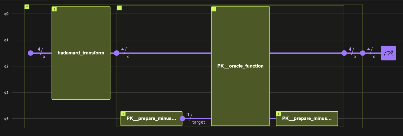
Therefore, the phase kickback primitive is constructed by the following steps:
-
Initializing the
qnumtype with \(4\) qubits using theallocatefunction such that \(| x \rangle=|0\rangle\). -
Applying the Hadamard transform using the
hadamard_transformfunction such that \(| x \rangle = \frac{1}{\sqrt{2^n}}\sum_{i=0}^{2^n-1}| i \rangle_n\). -
Applying the phase kickback primitive with the
oracle_phase_kickbackfunction such that \(| x \rangle = \frac{1}{\sqrt{2^n}}\sum_{i=0}^{2^n-1}(-1)^{i==0}| i \rangle_n\).
@qfunc
def main(x: Output[QNum]):
    allocate(num_qubits=4, out=x)
    hadamard_transform(x)
    oracle_phase_kickback(x)


qmod = create_model(main)
qprog = synthesize(qmod)
show(qprog)
Opening: https://platform.classiq.io/circuit/2uG1tsBMFj1MHSPifo9RQW60wUB?version=0.70.0
Verify that the quantum program actually operates as expected; receiving a minus \((-)\) phase only for the state \(|0\rangle\), that is: \(\begin{equation} | x \rangle = \frac{1}{\sqrt{2^4}}(|1\rangle+| 2 \rangle+\dots +| 15 \rangle-|0\rangle) \end{equation}\) To check, use the built-in Classiq state vector simulator from the IDE:
Indeed, we receive the minus \((-)\) phase only for the zero state, as expected.
The result shows bit strings of five bits rather than just four. This includes the target qubit measurement that always results in 0.
To see how this phase kickback is actually implemented in practice see the Deutsch-Josza example and Simon's example.
Mathematical Description
The starting point is the definition \(\begin{equation} O_f (| x \rangle_n| y \rangle_1) = | x \rangle_n|y \oplus f(x)\rangle_1 \end{equation}\) for \(f:\{0,1\}^n \rightarrow \{0,1\}\).
Applying \(O_f\) on \(| x \rangle| - \rangle\) results in this: \(\begin{equation} O_f (| x \rangle| - \rangle) = \frac{1}{\sqrt{2}}(| x \rangle |0 \oplus f(x)\rangle - | x \rangle |1 \oplus f(x)\rangle) \end{equation}\)
The expression \(0 \oplus f(x)\) equals \(f(x)\) because \(0\oplus0=0\) and \(0\oplus1=1\).
The expression \(1\oplus f(x)\) equals \(\overline{f(x)}\); i.e., NOT \(f(x)\) since \(1\oplus1=0\) and \(1\oplus0=1\).
Therefore:
\(\begin{equation} O_f (| x \rangle| - \rangle) = | x \rangle\frac{1}{\sqrt{2}}(|f(x)\rangle - |\overline{f(x)}\rangle). \end{equation}\)
If \(f(x)=0\) the target state is \(\frac{1}{\sqrt{2}}(|0\rangle - |1\rangle) = | - \rangle = (-1)^{f(x)}| - \rangle\).
If \(f(x)=1\) the target state is \(\frac{1}{\sqrt{2}}(|1\rangle - |0\rangle) = -| - \rangle = (-1)^{f(x)}| - \rangle\).
Therefore:
\(\begin{equation} O_f (| x \rangle| - \rangle) = (-1)^{f(x)}| x \rangle| - \rangle. \end{equation}\)
All the Code Together
Python version:
from classiq import *


@qfunc
def prepare_minus(target: Output[QBit]):
    allocate(out=target, num_qubits=1)
    X(target)
    H(target)


@qfunc
def oracle_function(target: QBit, x: QNum):
    target ^= x == 0


@qfunc
def oracle_phase_kickback(x: QNum):
    target = QBit("target")
    within_apply(
        within=lambda: prepare_minus(target), apply=lambda: oracle_function(target, x)
    )


@qfunc
def main(x: Output[QNum]):
    allocate(num_qubits=4, out=x)
    hadamard_transform(x)
    oracle_phase_kickback(x)


qmod = create_model(main, out_file="phase_kickback")
qprog = synthesize(qmod)
show(qprog)
Opening: https://platform.classiq.io/circuit/2uG1uFdW5FHb7CTWMfDW57ucXeh?version=0.70.0
References
[1]: Lecture Notes on Quantum Algorithms (Andrew M. Childs)
[2]: Lecture Notes on Quantum Algorithms for Scientific Computations (Lin Lin)
[3]: Quantum Computing: Lecture Notes (Ronald de Wolf)
[4]: Quantum Computation and Quantum Information (Michael Nielsen and Isaac Chuang)