The control statement applies a unitary operation conditionally, depending on a quantum state, and optionally a different one if the condition doesn’t hold. The unitary operations are specified as nested statement blocks. The objects used in the statement blocks become entangled with the object used in the condition, so that any superposition in the state of the condition carries over to the operations in the statement blocks. The control statement could be viewed as the quantum equivalent of the classical if statement, with a then block and an optional else block. The condition can be specified in one of two forms: as a single quantum variable, and as a quantum logical expression.Documentation Index
Fetch the complete documentation index at: https://prod-mint.classiq.io/llms.txt
Use this file to discover all available pages before exploring further.
Syntax
- Python
- Native
Semantics
- ctrl-var (in the first variant) is a quantum variable of type
qbitorqbit[], and ctrl-expression (in the second variant) is a logical expression over a quantum variable. - The statement block is applied if all the qubits in ctrl are in state (in the
first variant), or if the ctrl-expression evaluates to
true(in the second variant). - else-statements block is optional, and is applied if the negation of the condition holds, that is, if at least one of the qubits in ctrl is in state (in the first variant), or if the ctrl-expression evaluates to False (in the second variant).
- Currently, there exists a single limitation on the expression: if ctrl-expression is an equality between a single
variable and a classical expression, it is restricted to integers, meaning:
In a ctrl-expression of the form
<var> == <classical-expression>,<var>should be aqnumwith zero fraction places or aqbit, and<classical-expression>should evaluate to an integer. - The same variable cannot occur both in the condition and inside the statement block. This restriction applies also to mutually exclusive slices of the same variable.
- Quantum variables declared outside the control statement and used in its condition or inside its nested block must be initialized prior to it and remain initialized subsequently.
- Quantum variables declared inside the control statement, including in nested function calls, must be uninitialized at the end of the statement.
Examples
Example 1: Single-qubit control
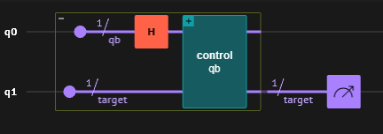
In the following example,control statement applies function X on the variable target
conditioned on a single qubit variable qb. Note that this is equivalent to using the
built-in gate-level function CX.
- Python
- Native

Example 2: Multi-qubit control
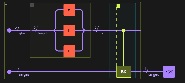
The next example shows howcontrol can be similarly used with multi-qubit control
variable. In this case target is rotated when the state of qba is the bit string 111.
- Python
- Native

Example 3: Numeric equality condition
The following example demonstrates the use ofcontrol to rotate the state of a qubit
by an angle determined by another quantum variable. In this case the condition compares
the quantum variable with the repeat index.
- Python
- Native
control
is implemented as positive and negative controls in the respective numeric qubits.

Example 4: Arithmetic condition
The following example demonstrates the use ofcontrol to rotate the state of a qubit
according to a condition imposed by another two quantum variables, x and y. Here, the condition
filters quantum states such that y <= x[0] + x[1] + x[2].
- Python
- Native
control
is implemented as a result of an arithmetic computation. After applying the control operation,
the arithmetic operation is uncomputed.

Example 5: Control else
The following example demonstrates the use of theelse block in the control statement.
In this case, the else block applies an ‘H’ gate on the target qubit when the control
condition is not met, instead of the ‘X’ gate,
so when each qubit of the control variable is in state , the bit is flipped,
otherwise, the Hadamard gate is applied.
- Python
- Native
else block
is implemented as a negation of the control condition, and the negation is uncomputed after
the control operation of the else block.


