Simon's Algorithm
Simon's algorithm [1], [2] is a basic quantum algorithm that demonstrates an exponential speed-up\(^*\) over its classical counterpart in the oracle complexity setting. The algorithm solves the so-called Simon's problem:
The algorithm treats the following problem:
- Input: A function \(f: [0,1]^n \rightarrow [0,1]^n\).
- Promise: There is a secret binary string \(s\) such that \(f(x) = f(y) \iff y = x\oplus s\tag{1}~~,\) where \(\oplus\) is a bitwise xor operation.
- Output: The secret string \(s\), using a minimal number of queries of \(f\).
Complexity: The Simon's problem is hard to solve with classical deterministic or probabalistic approaches. This can be understood as follows: determining \(s\) requires finding a collision \(f(x)=f(y)\), as \(s = x\oplus y\). What is the minimum number of calls for measuring a collision? If we take the deterministic approach, in the worst case we need \(2^{n-1}\) calls. A probablistic approach, in the spirit of the one that solves the birthday problem [3], has slightly better scaling of \(O(2^{n/2})\) queries. The quantum approach requires \(O(n)\) queries, thus introducing an exponential speedup.
\(^*\) The exponential speedup is in the oracle complexity setting. It only refers to deterministic classical machines.
Keywords: Foundational quantum algorithm, Exponential speedup, Function evaluation, Oracle problem, Oracle/Query complexity.
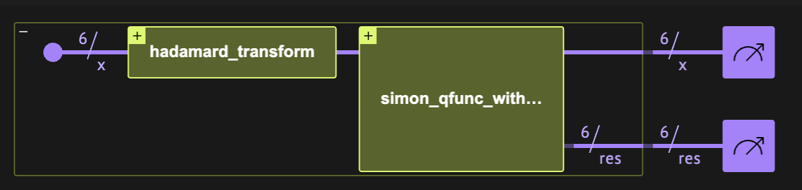
Figure 1. The Simon's algorithm comprises two quantum blocks. The main part of the algorithm is the oracle that implements the Simon's function f(x).
In the following notebook we define the Simon's algorithm, which has a quantum part and a classical postprocess part. Then, we run the algorithm on two different examples of a Simon's function: one that can be defined with simple arithmetic and another that has a shallow implementation. A mathematical explanation of the algorithm is provided at the end of this notebook.
Note that the function \(f\) is \(2\)-to-\(1\) if \(s\neq 0^n\), and \(1\)-to-\(1\) otherwise. Hereafter, we refer to a function that satisfies the condition in Eq. (1) as a "Simon's function".
Building the Algorithm with Classiq
Quantum Part
The quantum part of the algorithm is rather simple, calling the quantum implementation of \(f(x)\), between two calls of the hadamard transform. The call of \(f\) is done out-of-place, onto a quantum variable \(res\), whereas only the final state of \(x\) is relevant to the classical postprocess to follow.
from classiq import *


@qfunc
def simon_qfunc(f_qfunc: QCallable[QNum, Output[QNum]], x: QNum, res: Output[QNum]):
    within_apply(lambda: hadamard_transform(x), lambda: f_qfunc(x, res))
Classical Postprocess
The classical part of the algorithm includes the following postprocessing steps:
-
Finding \(n-1\) samples of \(x\) that are linearly independent, \(\{y_k\}^{n-1}_{1}\). It is guaranteed that this can be achieved with high probability (see the technical details below).
-
Finding the string \(s\) such that \(s \cdot y_k=0 \,\,\, \forall k\), where \(\cdot\) refers to a dot-product \(\text{mod}~ 2\) (polynomial complexity in \(n\)).
For these steps we use the Galois package, which extends NumPy to finite field operations.
# !pip install galois
import galois
import numpy as np

# here we work over Boolean arithmetics - F(2)
GF = galois.GF(2)
We define two classical functions for the first step:
# The following function checks whether a set contains linearly independent vectors


def is_independent_set(vectors):
    matrix = GF(vectors)
    rank = np.linalg.matrix_rank(matrix)
    if rank == len(vectors):
        return True
    else:
        return False


def get_independent_set(samples):
    """
    The following function gets samples of n-sized strings from running the quantum part and returns an n-1 x n matrix,
    whose rows form a set if independent.
    """
    ind_v = []
    for v in samples:
        if is_independent_set(ind_v + [v]):
            ind_v.append(v)
            if len(ind_v) == len(v) - 1:
                # reached max set of N-1
                break
    return ind_v
For the second step we need to solve a linear set of equations. We have \(n-1\) equations on a binary vector of size \(n\). It has two solutions, one of which is the trivial solution \(0^n\), while the other gives us the secret string \(s\). The Galois package handles this task as follows:
def get_secret_integer(matrix):
    """
    Finds a binary vector that “solves” the equation
    Ax=0 (mod 2) —
    and then turns that vector into a single integer, which serves as the “secret”.
    """
    gf_v = GF(matrix)  # converting to a matrix over Z_2
    null_space = gf_v.T.left_null_space()  # finding the right-null space of the matrix
    return int(
        "".join(np.array(null_space)[0][::-1].astype(str)), 2
    )  # converting from binary to integer
Next, we provide two different examples of Simon's function and run the Simon's algorithm to find their secret string.
Example: Arithmetic Simon's Function
An example of a valid \(f(x)\) function that satisfies the condition in Eq. (1):
Clearly, we have that \(f(x\oplus s) = \min(x\oplus s, (x\oplus s)\oplus s)=\min(x\oplus s, x)=f(x)\).
Implementing the Simon's Function
We define the function, as well as a model that applies it on all computational basis states to illustrate that it is a two-to-one function.
from classiq.qmod.symbolic import min


@qperm
def simon_qfunc_simple(s: CInt, x: Const[QNum], res: Output[QNum]):
    res |= min(x, x ^ s)
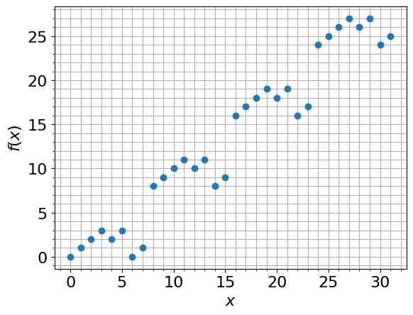
Let us run it with \(n=5\) and \(s={'}00110{'} (\equiv 6)\), starting with a uniform distribution of \(|x\rangle\) over all possible states:
NUM_QUBITS = 5
S_SECRET = 6


@qfunc
def main(x: Output[QNum[NUM_QUBITS]], res: Output[QNum]):
    allocate(x)
    hadamard_transform(x)
    simon_qfunc_simple(S_SECRET, x, res)


qmod_1 = create_model(main)

# synthesize
qprog_1 = synthesize(
    qmod_1, constraints=Constraints(optimization_parameter=OptimizationParameter.WIDTH)
)
# vizualize
show(qprog_1)

# execute
result_1 = execute(qprog_1).result_value()
Quantum program link: https://platform.classiq.io/circuit/34mXZB9OZkWeWOpIZVwXMziie2v
By plotting the results we can see that this is a two-to-one function:
import matplotlib.pyplot as plt

my_result = {
    sample.state["x"]: sample.state["res"] for sample in result_1.parsed_counts
}
fig, ax = plt.subplots()
ax.plot(my_result.keys(), my_result.values(), "o")
ax.grid(axis="y", which="minor")
ax.grid(axis="y", which="major")
ax.grid(axis="x", which="minor")
ax.grid(axis="x", which="major")
plt.xlabel("$x$", fontsize=16)
plt.ylabel("$f(x)$", fontsize=16)
plt.yticks(fontsize=16)
plt.xticks(fontsize=16)
ax.minorticks_on()
Running the Simon's Algorithm
Taking \(n\) number of shots guarantees getting a set of \(n-1\) independent strings with high probability (assuming a noiseless quantum computer) (see technical explanation below). Moreover, increasing the number of shots by a constant factor provides an exponential improvement. Here we take \(50*n\) shots.
from classiq.execution import ExecutionPreferences


@qfunc
def main(x: Output[QNum[NUM_QUBITS]], res: Output[QNum]):
    allocate(x)
    simon_qfunc(lambda x, res: simon_qfunc_simple(S_SECRET, x, res), x, res)


qmod_2 = create_model(
    main,
    constraints=Constraints(optimization_parameter=OptimizationParameter.WIDTH),
    # execution_preferences=ExecutionPreferences(num_shots=50 * NUM_QUBITS),
    out_file="simon",
)
We synthesize and execute to obtain the results:
qprog_2 = synthesize(qmod_2)

# increasing the number of shots
prefs_more_shots = ExecutionPreferences(num_shots=50 * NUM_QUBITS)
with ExecutionSession(qprog_2, execution_preferences=prefs_more_shots) as es:
    result_2 = es.sample()

bitstrings = [f"{x:0{NUM_QUBITS}b}" for x in result_2.dataframe["x"].tolist()]
reversed_bitstrings = [b[::-1] for b in bitstrings]
samples = [[int(bit) for bit in b] for b in reversed_bitstrings]
matrix_of_ind_v = get_independent_set(samples)
assert (
    len(matrix_of_ind_v) == NUM_QUBITS - 1
), "Failed to find an independent set, try to increase the number of shots"
quantum_secret_integer = get_secret_integer(matrix_of_ind_v)
print("The secret binary string (integer) of f(x):", S_SECRET)
print("The result of the Simon's Algorithm:", quantum_secret_integer)
assert (
    S_SECRET == quantum_secret_integer
), "The Simon's algorithm failed to find the secret key."
The secret binary string (integer) of f(x): 6
The result of the Simon's Algorithm: 6
Example: Shallow Simon's Function
In the second example we take a Simon's function that was presented in a recent paper [4]: Take a secret string of the form \(s=0^{n-l}1^l = \underbrace{00\dots0}_{n-l}\underbrace{1\dots111}_{l}~,\) and define the 2-to-1 function:
The function \(f\) operates as follows: for the first \(n-l\) elements, we simply "copy" the data, whereas for the last \(l\) elements we apply a xor with the \(n-l\) element. A simple proof that this is indeed a 2-to-1 function is given in Ref. [4].
Comment: Ref. [4] employed further reduction of the function implementation (reducing the \(n\)-sized Simon's problem to an \((n-l)\)-sized problem), added a classical postprocess of randomly permutating over the result of \(f(x)\) to increase the hardness of the problem, and also included some NISQ analysis. These steps were taken to show an algorithmic speedup on real quantum hardware.
Implementing the Simon's Function
The first \(n-l\) "classical copies", \(|x_k,0\rangle\rightarrow |x_k x_k\rangle\), can be implemented by \(CX\) gates. The xor operations, \(|x_k,0\rangle\rightarrow |x_k, x_k \oplus x_{n-l}\rangle\), can be implemented by two \(CX\) operations, one to form a "classical copy" of \(x_k\), followed by another \(CX\) operation, implementing a xor with \(x_{n-l}\).
@qperm
def simon_qfunc_with_bipartite_s(
    partition_index: CInt, x: Const[QArray], res: Output[QArray]
):
    allocate(x.len, res)

    repeat(x.len - partition_index, lambda i: CX(x[i], res[i]))
    repeat(
        partition_index - 1,
        lambda i: (
            CX(
                x[x.len - partition_index + 1 + i],
                res[x.len - partition_index + 1 + i],
            ),
            CX(x[x.len - partition_index], res[x.len - partition_index + 1 + i]),
        ),
    )
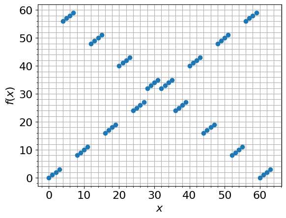
Here we take a specific example and plot \(f(x)\) for all possible \(x\) values:
NUM_QUBITS = 6
PARTITION_INDEX = 4


@qfunc
def main(x: Output[QNum[NUM_QUBITS]], res: Output[QNum]):
    allocate(x)
    hadamard_transform(x)
    simon_qfunc_with_bipartite_s(PARTITION_INDEX, x, res)


# create model
qmod_3 = create_model(main)
# synthesize
qprog_3 = synthesize(
    qmod_3, constraints=Constraints(optimization_parameter=OptimizationParameter.DEPTH)
)
# vizualize
show(qprog_3)

# execute
result_3 = execute(qprog_3).result_value()

# plot the f(x)
my_result = {
    sample.state["x"]: sample.state["res"] for sample in result_3.parsed_counts
}
fig, ax = plt.subplots()
ax.plot(my_result.keys(), my_result.values(), "o")
ax.grid(axis="y", which="minor")
ax.grid(axis="y", which="major")
ax.grid(axis="x", which="minor")
ax.grid(axis="x", which="major")
plt.xlabel("$x$", fontsize=16)
plt.ylabel("$f(x)$", fontsize=16)
plt.yticks(fontsize=16)
plt.xticks(fontsize=16)
ax.minorticks_on()
Quantum program link: https://platform.classiq.io/circuit/34mXayl4zIuAmxIjnE4RBKh6W6e
Running the Simon's Algorithm
As in the first example, we take \(50*n\) shots.
@qfunc
def main(x: Output[QNum[NUM_QUBITS]], res: Output[QNum]):
    allocate(x)
    simon_qfunc(
        lambda x, res: simon_qfunc_with_bipartite_s(PARTITION_INDEX, x, res), x, res
    )


qmod_4 = create_model(main)
# qmod_4 = update_execution_preferences(qmod_4, num_shots=50 * NUM_QUBITS)
We synthesize and execute to obtain the results:
qprog_4 = synthesize(qmod_4)
show(qprog_4)

# increasing the number of shots
prefs_more_shots = ExecutionPreferences(num_shots=50 * NUM_QUBITS)
with ExecutionSession(qprog_4, execution_preferences=prefs_more_shots) as es:
    result_4 = es.sample()

bitstrings = [f"{x:0{NUM_QUBITS}b}" for x in result_4.dataframe["x"].tolist()]
reversed_bitstrings = [b[::-1] for b in bitstrings]
samples = [[int(bit) for bit in b] for b in reversed_bitstrings]
Quantum program link: https://platform.classiq.io/circuit/34mXbMMLtk1sPiueLNiSsdYPRwP
matrix_of_ind_v = get_independent_set(samples)
assert (
    len(matrix_of_ind_v) == NUM_QUBITS - 1
), "Failed to find an independent set, try to increase the number of shots"
quantum_secret_integer = get_secret_integer(matrix_of_ind_v)
s_secret = int("1" * PARTITION_INDEX + "0" * (NUM_QUBITS - PARTITION_INDEX), 2)
print("The secret binary string (integer) of f(x):", s_secret)
print("The result of the Simon's Algorithm:", quantum_secret_integer)
assert (
    s_secret == quantum_secret_integer
), "The Simon's algorithm failed to find the secret key."
The secret binary string (integer) of f(x): 60
The result of the Simon's Algorithm: 60
Technical Notes
This section provides some technical details about the quantum and classical parts of the Simon's algorithm.
Quantum Part
Following the three blocks of the algorithm:
We next measure the first register \(|y\rangle\). First, we treat the case where \(s\neq 0\) that \(f(x)\) is a 2-to-1 function. The claim is that for any measured state \(y\), we must have that \(y\cdot s=0\). To see this, calculate the probability of measuring some state \(|y\rangle\):
Now, change the sum to run over the image of \(f(x)\) instead of over all \(x\in [0,2^{n}-1]\). Since for any \(f(x)\) there are two sources in the domain, \(x\) and \(x\oplus s\), we can write
Since $\((-1)^{x\cdot y} + (-1)^{(x\oplus s )\cdot y} = (-1)^{x\cdot y}( 1+ (-1)^{s\cdot y})\)$ vanishes when \(s\cdot y \neq 0 ~(\text{mod}~ 2)\), for any measured \(y\) we have \(y\cdot s = 0\). Therefore, every measurement \(y\) gives a random vector orthogonal to \(s\). Repeating \(O(n)\) measurements collects \(n-1\) linear modular equations which span the orthogonal space to \(s\).
Classical Part
We have a set of possible \(y\) values that can be measured, each with a probability of \(1/M\), where \(M\) is the set size. If \(s=0^n\), we have \(M=2^n\), whereas for \(s\neq 0^n\) the set size is \(M=2^{n-1}\). The probability of measuring a set of \(n-1\) linearly independent binary strings \(y\) can be calculated as follows (see also the birthday problem [2]): For the first string, \(y_0\), we just require that we do not pick \(y=0^n\), so \(P(y_0)=1-1/M\). Then, for the next string, we require that it is not in \(\left\{a_0 y_0\,\,\,| a_0=0,1\right\}\), thus \(P(y_1)=(1-2/M)\). The following string must not be picked out of \(\left\{a_0 y_0+a_1y_1\,\,\,| a_0, a_1=0,1\right\}\), thus \(P(y_2)=(1-2^2/M)\). We can continue with this procedure up to \(y_{n-2}\) (in total \(n-1\) vectors) to get
If we repeat the experiment, the probability of measuring an independent set improves exponentially. Solving the linear system recovers \(s\).
Reference
[1] Simon, D. R. (1997). On the power of quantum computation. SIAM journal on computing, 26(5), 1474-1483.
[2] Simon's Algorithm (Wikipedia).
[4] Singkanipa P. et al. Demonstration of Algorithmic Quantum Speedup for an Abelian Hidden Subgroup Problem.