Discrete Logarithm

View on GitHub Experiment in the IDE

The Discrete Logarithm Problem [1] was shown by Shor [2] to be solved in a polynomial time using quantum computers, while the fastest classical algorithms take a superpolynomial time. The problem is at least as hard as the factoring problem. In fact, the hardness of the problem is the basis for the Diffie-Hellman [3]] protocol for key exchange.

Problem formulation

Input: A cyclic group $G = \langle g \rangle$ with $g$ as a generator, and an element $x\in G$.
Promise: There is a number $s$ such that $g^s = x$.
Output: $s$, the discrete logarithm: $s = \log_gx$

In Shor's implementation the order of $g$ is assumed to be known beforehand (for example using the order finding algorithm). We will also assume it in the demonstration.

The Discrete Log problem is a specific example for the Abelian Hidden Subgroup Problem [4], for the case where G is the additive group $\mathbb{Z}_N \times \mathbb{Z}_N$, with the function:

\[f(\alpha, \beta) = x^\alpha g^\beta\]

How to build the Algorithm with Classiq

The heart of the algorithm's logic is the implementation of the function:

\[|x_1\rangle|x_2\rangle|1\rangle \rightarrow |x_1\rangle|x_2\rangle|x^{x_1} g^{x_2}\rangle\]

This is done using 2 applications of the modular exponentiation function, which was described in detail in the Shor's Factoring Algorithm notebook. So here we will just import it from the classiq's library.

The function modular_exp accepts the following arguments:

n: CInt - modulo number
a: CInt - base of the exponentiation
x: QArray[QBit] - unsigned integer to multiply be the exponentiation
power: QArray[QBit]- power of the exponentiation

So that the function implements: $|power\rangle|x\rangle \rightarrow |power\rangle|x \cdot a ^ {power}\mod n\rangle$

from classiq.qmod import (
    CInt,
    Output,
    QArray,
    QBit,
    QNum,
    allocate,
    inplace_prepare_int,
    modular_exp,
    qfunc,
)


@qfunc
def discrete_log_oracle(
    g_generator: CInt,
    x_element: CInt,
    N_modulus: CInt,
    order: CInt,
    x1: QArray[QBit],
    x2: QArray[QBit],
    func_res: Output[QArray[QBit]],
) -> None:

    allocate(ceiling(log(N_modulus, 2)), func_res)

    inplace_prepare_int(1, func_res)
    modular_exp(N_modulus, x_element, func_res, x1)
    modular_exp(N_modulus, g_generator, func_res, x2)

The full algorithm:

Prepare uniform superposition over the first 2 quantum variables x1, x2. Each variable should be with size $\lceil \log r\rceil + \log({1/{\epsilon}})$. In the special case where $r$ is a power of 2, $\log r$ is enough.
Compute discrete_log_oracle on the func_res variable. func_res should be of size $\lceil \log N\rceil$.
Apply inverse Fourier transform x1, x2.
Measure.

from classiq.qmod import hadamard_transform, invert, qft
from classiq.qmod.symbolic import ceiling, log


@qfunc
def discrete_log(
    g: CInt,
    x: CInt,
    N: CInt,
    order: CInt,
    x1: Output[QArray[QBit]],
    x2: Output[QArray[QBit]],
    func_res: Output[QArray[QBit]],
) -> None:
    reg_len = ceiling(log(order, 2))
    allocate(reg_len, x1)
    allocate(reg_len, x2)

    hadamard_transform(x1)
    hadamard_transform(x2)

    discrete_log_oracle(g, x, N, order, x1, x2, func_res)

    invert(lambda: qft(x1))
    invert(lambda: qft(x2))

After the inverse QFTs, we get in the variables (under the assumption of $r=2^m$ for some $m$):

\[|\psi\rangle = \sum_{\nu\in\mathbb{Z}_r, \delta\in G}\omega^{\nu\delta}|\nu log_gx\rangle_{x_1}|\nu\rangle_{x_2}|\delta>_{func\_res}\]

For every $\nu$ that has a mutplicative inverse in $\mathbb{Z}_r$, we can extract $s=\log_xg$ by multiplying the first variable result by its inverse.

In the case where $r$ is not a power of 2, we get in the variables and approximation of: |$ \log_g(x) \nu/ r\rangle_{x_1} |\nu / r\rangle_{x_2}$. So we can use the continued fractions algorithm [5] to compute $\nu/r$, then using the same technique to calculate $\log_gx$.

Note: Alternatively, one might implement the $QFT_{\mathbb{Z}_r}$ over general $r$, and instead of the uniform superposition prepare the states: $\frac{1}{\sqrt{r}}\sum_{x\in\mathbb{r}}|x\rangle$ in x1, x2. Then again no continued fractions post-process is required.

Example: $G = \mathbb{Z}_5^\times$

For this specific demonstration, we choose $G = \mathbb{Z}_5^\times$, with $g=3$ and $x=2$. Under this setting, $log_gx=3$.

We choose this specific example as the order of of the group $r=4$ is a power of $2$, and so we can get exactly the discrete logarithm, without continued-fractions post processing. In other cases, one has to use larger quantum variable for the exponents so the continued fractions post-processing will converge.

from classiq import Constraints, create_model

MODULU_NUM = 5
G_GENERATOR = 3
X_LOGARITHM = 2
ORDER = MODULU_NUM - 1  # as 5 is prime


@qfunc
def main(
    x1: Output[QNum],
    x2: Output[QNum],
    func_res: Output[QNum],
) -> None:
    discrete_log(G_GENERATOR, X_LOGARITHM, MODULU_NUM, ORDER, x1, x2, func_res)

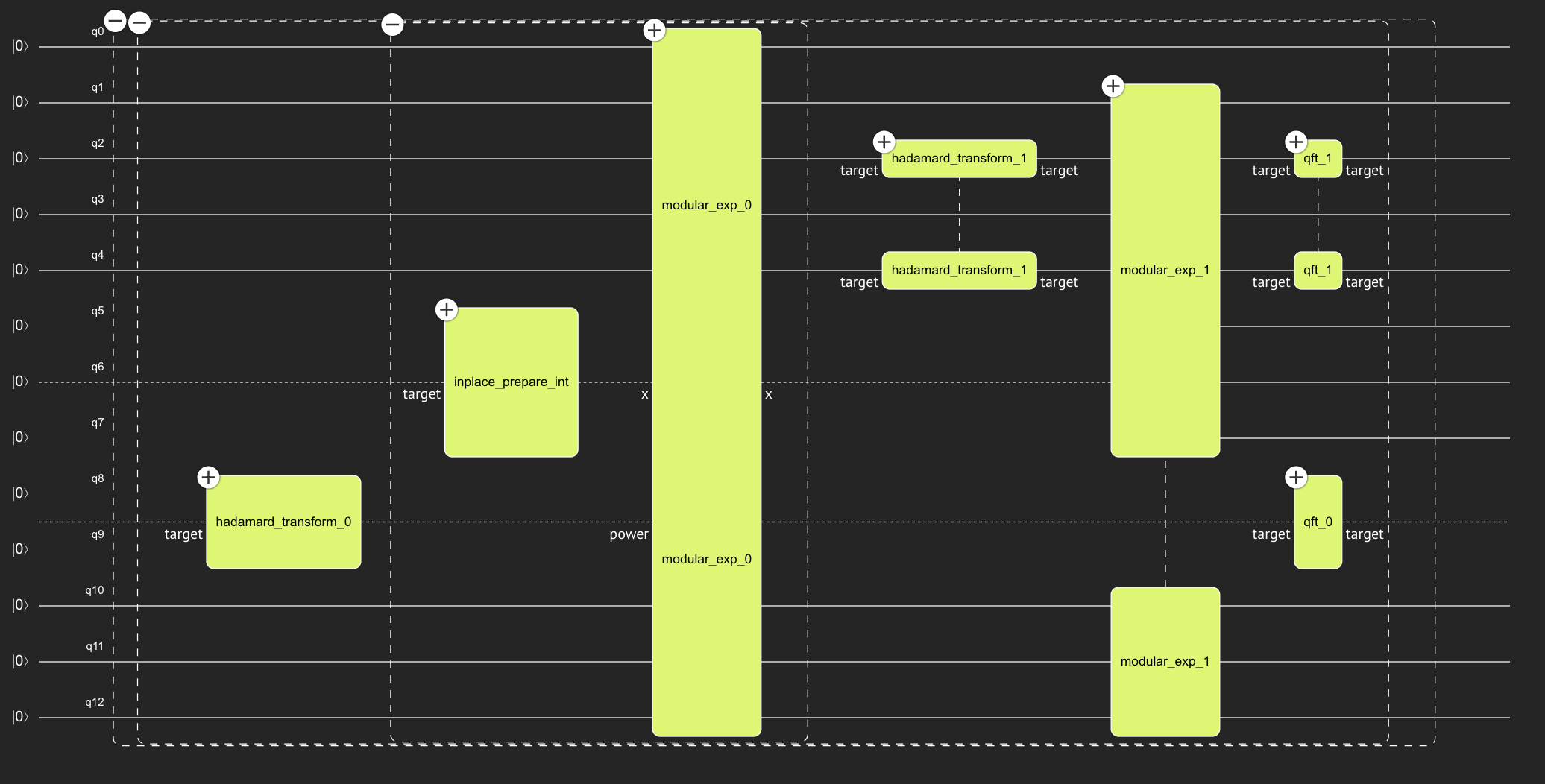
from classiq import Preferences, show, synthesize, write_qmod

constraints = Constraints(max_width=13)
qmod = create_model(main, constraints=constraints)
write_qmod(qmod, "discrete_log")

qprog = synthesize(qmod)
show(qprog)

Opening: http://localhost:4200/circuit/41ec5ffb-0221-449a-962a-a438c8c1a193?version=0.0.0

from classiq import execute

results = execute(qprog).result()
res = results[0].value
res.parsed_counts

[{'x1': 3.0, 'x2': 1.0, 'func_res': 4.0}: 79,
 {'x1': 1.0, 'x2': 3.0, 'func_res': 1.0}: 67,
 {'x1': 0.0, 'x2': 0.0, 'func_res': 1.0}: 66,
 {'x1': 2.0, 'x2': 2.0, 'func_res': 3.0}: 66,
 {'x1': 0.0, 'x2': 0.0, 'func_res': 2.0}: 66,
 {'x1': 0.0, 'x2': 0.0, 'func_res': 3.0}: 66,
 {'x1': 2.0, 'x2': 2.0, 'func_res': 2.0}: 64,
 {'x1': 1.0, 'x2': 3.0, 'func_res': 2.0}: 63,
 {'x1': 2.0, 'x2': 2.0, 'func_res': 4.0}: 62,
 {'x1': 3.0, 'x2': 1.0, 'func_res': 1.0}: 62,
 {'x1': 3.0, 'x2': 1.0, 'func_res': 2.0}: 61,
 {'x1': 0.0, 'x2': 0.0, 'func_res': 4.0}: 60,
 {'x1': 1.0, 'x2': 3.0, 'func_res': 3.0}: 57,
 {'x1': 1.0, 'x2': 3.0, 'func_res': 4.0}: 56,
 {'x1': 3.0, 'x2': 1.0, 'func_res': 3.0}: 55,
 {'x1': 2.0, 'x2': 2.0, 'func_res': 1.0}: 50]

Notice that func_res is uncorrelated to the other variables, and we get uniform distribution, as expected.

We take only the x2 that are co-prime to $r=4$, so they have a multiplicative-inverse. Hence x2=1,3 are the relevant results. So we get 2 relevant results (for all different $\delta$s): $|1\rangle|3\rangle$, $|3\rangle|1\rangle$. All left to do to get the logarithm is to multiply x1 by the inverse of x2: