Max Colorable Induced Subgraph Problem
Background
Given a graph \(G = (V,E)\) and number of colors K, find the largest induced subgraph that can be colored using up to K colors.
A coloring is legal if:
-
each vetrex \({v_i}\) is assigned with a color \(k_i \in \{0, 1, ..., k-1\}\)
-
adajecnt vertex have different colors: for each \(v_i, v_j\) such that \((v_i, v_j) \in E\), \(k_i \neq k_j\).
An induced subgraph of a graph \(G = (V,E)\) is a graph \(G'=(V', E')\) such that \(V'\subset V\) and \(E' = \{(v_1, v_2) \in E\ |\ v_1, v_2 \in V'\}\).
Define the optimization problem
import networkx as nx
import numpy as np
import pyomo.environ as pyo


def define_max_k_colorable_model(graph, K):
    model = pyo.ConcreteModel()

    nodes = list(graph.nodes())
    colors = range(0, K)

    # each x_i states if node i belongs to the cliques
    model.x = pyo.Var(colors, nodes, domain=pyo.Binary)
    x_variables = np.array(list(model.x.values()))

    adjacency_matrix = nx.convert_matrix.to_numpy_array(graph, nonedge=0)
    adjacency_matrix_block_diagonal = np.kron(np.eye(K), adjacency_matrix)

    # constraint that 2 nodes sharing an edge mustn't have the same color
    model.conflicting_color_constraint = pyo.Constraint(
        expr=x_variables @ adjacency_matrix_block_diagonal @ x_variables == 0
    )

    # each node should be colored
    @model.Constraint(nodes)
    def each_node_is_colored_once_or_zero(model, node):
        return sum(model.x[color, node] for color in colors) <= 1

    def is_node_colored(node):
        is_colored = np.prod([(1 - model.x[color, node]) for color in colors])
        return 1 - is_colored

    # maximize the number of nodes in the chosen clique
    model.value = pyo.Objective(
        expr=sum(is_node_colored(node) for node in nodes), sense=pyo.maximize
    )

    return model
Initialize the model with parameters
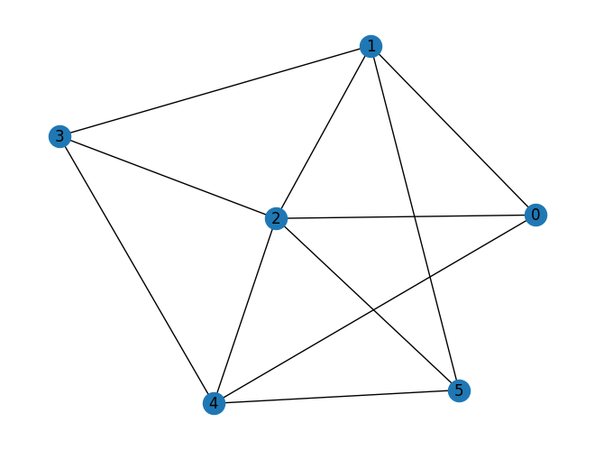
graph = nx.erdos_renyi_graph(6, 0.5, seed=7)
nx.draw_kamada_kawai(graph, with_labels=True)

NUM_COLORS = 2

coloring_model = define_max_k_colorable_model(graph, NUM_COLORS)
print the resulting pyomo model
coloring_model.pprint()
4 Set Declarations
    each_node_is_colored_once_or_zero_index : Size=1, Index=None, Ordered=Insertion
        Key  : Dimen : Domain : Size : Members
        None :     1 :    Any :    6 : {0, 1, 2, 3, 4, 5}
    x_index : Size=1, Index=None, Ordered=True
        Key  : Dimen : Domain              : Size : Members
        None :     2 : x_index_0*x_index_1 :   12 : {(0, 0), (0, 1), (0, 2), (0, 3), (0, 4), (0, 5), (1, 0), (1, 1), (1, 2), (1, 3), (1, 4), (1, 5)}
    x_index_0 : Size=1, Index=None, Ordered=Insertion
        Key  : Dimen : Domain : Size : Members
        None :     1 :    Any :    2 : {0, 1}
    x_index_1 : Size=1, Index=None, Ordered=Insertion
        Key  : Dimen : Domain : Size : Members
        None :     1 :    Any :    6 : {0, 1, 2, 3, 4, 5}

1 Var Declarations
    x : Size=12, Index=x_index
        Key    : Lower : Value : Upper : Fixed : Stale : Domain
        (0, 0) :     0 :  None :     1 : False :  True : Binary
        (0, 1) :     0 :  None :     1 : False :  True : Binary
        (0, 2) :     0 :  None :     1 : False :  True : Binary
        (0, 3) :     0 :  None :     1 : False :  True : Binary
        (0, 4) :     0 :  None :     1 : False :  True : Binary
        (0, 5) :     0 :  None :     1 : False :  True : Binary
        (1, 0) :     0 :  None :     1 : False :  True : Binary
        (1, 1) :     0 :  None :     1 : False :  True : Binary
        (1, 2) :     0 :  None :     1 : False :  True : Binary
        (1, 3) :     0 :  None :     1 : False :  True : Binary
        (1, 4) :     0 :  None :     1 : False :  True : Binary
        (1, 5) :     0 :  None :     1 : False :  True : Binary

1 Objective Declarations
    value : Size=1, Index=None, Active=True
        Key  : Active : Sense    : Expression
        None :   True : maximize : 1 - (1 - x[0,0])*(1 - x[1,0]) + 1 - (1 - x[0,1])*(1 - x[1,1]) + 1 - (1 - x[0,2])*(1 - x[1,2]) + 1 - (1 - x[0,3])*(1 - x[1,3]) + 1 - (1 - x[0,4])*(1 - x[1,4]) + 1 - (1 - x[0,5])*(1 - x[1,5])

2 Constraint Declarations
    conflicting_color_constraint : Size=1, Index=None, Active=True
        Key  : Lower : Body                                                                                                                                                                                                                                                                                                                                                                                                                                                                                                                  : Upper : Active
        None :   0.0 : (x[0,1] + x[0,2] + x[0,4])*x[0,0] + (x[0,0] + x[0,2] + x[0,3] + x[0,5])*x[0,1] + (x[0,0] + x[0,1] + x[0,3] + x[0,4] + x[0,5])*x[0,2] + (x[0,1] + x[0,2] + x[0,4])*x[0,3] + (x[0,0] + x[0,2] + x[0,3] + x[0,5])*x[0,4] + (x[0,1] + x[0,2] + x[0,4])*x[0,5] + (x[1,1] + x[1,2] + x[1,4])*x[1,0] + (x[1,0] + x[1,2] + x[1,3] + x[1,5])*x[1,1] + (x[1,0] + x[1,1] + x[1,3] + x[1,4] + x[1,5])*x[1,2] + (x[1,1] + x[1,2] + x[1,4])*x[1,3] + (x[1,0] + x[1,2] + x[1,3] + x[1,5])*x[1,4] + (x[1,1] + x[1,2] + x[1,4])*x[1,5] :   0.0 :   True
    each_node_is_colored_once_or_zero : Size=6, Index=each_node_is_colored_once_or_zero_index, Active=True
        Key : Lower : Body            : Upper : Active
          0 :  -Inf : x[0,0] + x[1,0] :   1.0 :   True
          1 :  -Inf : x[0,1] + x[1,1] :   1.0 :   True
          2 :  -Inf : x[0,2] + x[1,2] :   1.0 :   True
          3 :  -Inf : x[0,3] + x[1,3] :   1.0 :   True
          4 :  -Inf : x[0,4] + x[1,4] :   1.0 :   True
          5 :  -Inf : x[0,5] + x[1,5] :   1.0 :   True

8 Declarations: x_index_0 x_index_1 x_index x conflicting_color_constraint each_node_is_colored_once_or_zero_index each_node_is_colored_once_or_zero value
Setting Up the Classiq Problem Instance
In order to solve the Pyomo model defined above, we use the Classiq combinatorial optimization engine. For the quantum part of the QAOA algorithm (QAOAConfig) - define the number of repetitions (num_layers):
from classiq import *
from classiq.applications.combinatorial_optimization import OptimizerConfig, QAOAConfig

qaoa_config = QAOAConfig(num_layers=8)
For the classical optimization part of the QAOA algorithm we define the maximum number of classical iterations (max_iteration) and the \(\alpha\)-parameter (alpha_cvar) for running CVaR-QAOA, an improved variation of the QAOA algorithm [3]:
optimizer_config = OptimizerConfig(max_iteration=20, alpha_cvar=0.7)
Lastly, we load the model, based on the problem and algorithm parameters, which we can use to solve the problem:
qmod = construct_combinatorial_optimization_model(
    pyo_model=coloring_model,
    qaoa_config=qaoa_config,
    optimizer_config=optimizer_config,
)
We also set the quantum backend we want to execute on:
from classiq.execution import ClassiqBackendPreferences

qmod = set_execution_preferences(
    qmod, backend_preferences=ClassiqBackendPreferences(backend_name="simulator")
)
write_qmod(qmod, "max_induced_k_color_subgraph")
Synthesizing the QAOA Circuit and Solving the Problem
We can now synthesize and view the QAOA circuit (ansatz) used to solve the optimization problem:
qprog = synthesize(qmod)
show(qprog)
Opening: https://platform.classiq.io/circuit/941213ad-27c1-464a-8fb9-3936559e6168?version=0.41.0.dev39%2B79c8fd0855
We now solve the problem by calling the execute function on the quantum program we have generated:
result = execute(qprog).result_value()
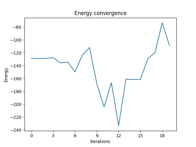
We can check the convergence of the run:
result.convergence_graph
Optimization Results
We can also examine the statistics of the algorithm:
import pandas as pd

from classiq.applications.combinatorial_optimization import (
    get_optimization_solution_from_pyo,
)

solution = get_optimization_solution_from_pyo(
    coloring_model, vqe_result=result, penalty_energy=qaoa_config.penalty_energy
)
optimization_result = pd.DataFrame.from_records(solution)
optimization_result.sort_values(by="cost", ascending=False).head(5)
| probability | cost | solution | count | |
|---|---|---|---|---|
| 401 | 0.001 | 5.0 | [1, 0, 0, 1, 0, 1, 0, 1, 0, 0, 1, 0] | 1 |
| 572 | 0.001 | 4.0 | [1, 0, 0, 1, 0, 1, 0, 0, 1, 0, 0, 0] | 1 |
| 334 | 0.001 | 3.0 | [1, 0, 0, 0, 0, 1, 0, 0, 0, 1, 0, 0] | 1 |
| 222 | 0.001 | 3.0 | [0, 0, 0, 0, 1, 0, 1, 0, 0, 0, 0, 1] | 1 |
| 169 | 0.001 | 3.0 | [0, 1, 0, 0, 0, 0, 1, 0, 0, 1, 0, 0] | 1 |
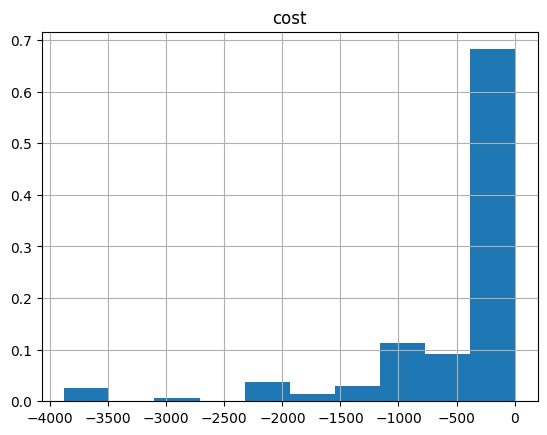
And the histogram:
optimization_result.hist("cost", weights=optimization_result["probability"])
array([[<Axes: title={'center': 'cost'}>]], dtype=object)
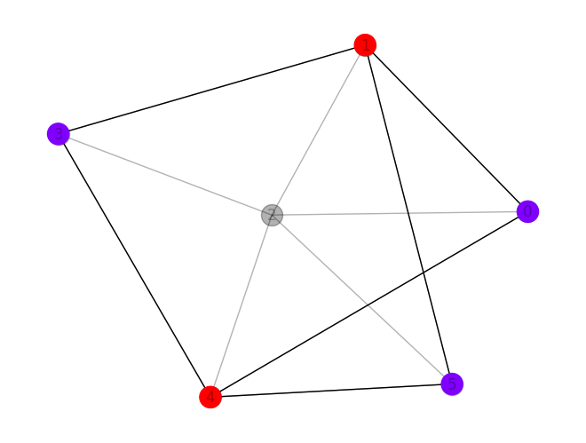
Let us plot the best solution:
import matplotlib.pyplot as plt

best_solution = optimization_result.solution[optimization_result.cost.idxmax()]

one_hot_solution = np.array(best_solution).reshape([NUM_COLORS, len(graph.nodes)])
integer_solution = np.argmax(one_hot_solution, axis=0)

colored_nodes = np.array(graph.nodes)[one_hot_solution.sum(axis=0) != 0]
colors = integer_solution[colored_nodes]

pos = nx.kamada_kawai_layout(graph)
nx.draw(graph, pos=pos, with_labels=True, alpha=0.3, node_color="k")
nx.draw(graph.subgraph(colored_nodes), pos=pos, node_color=colors, cmap=plt.cm.rainbow)
Classical optimizer results
Lastly, we can compare to the classical solution of the problem:
from pyomo.common.errors import ApplicationError
from pyomo.opt import SolverFactory

solver = SolverFactory("couenne")
result = None
try:
    result = solver.solve(coloring_model)
except ApplicationError:
    print("Solver might have not exited normally. Try again")

coloring_model.display()
ERROR: Solver (asl) returned non-zero return code (-6)


ERROR: Solver log: Couenne 0.5.8 -- an Open-Source solver for Mixed Integer
    Nonlinear Optimization Mailing list: couenne@list.coin-or.org
    Instructions: http://www.coin-or.org/Couenne malloc_consolidate(): invalid
    chunk size couenne:


Solver might have not exited normally. Try again
Model unknown

  Variables:
    x : Size=12, Index=x_index
        Key    : Lower : Value : Upper : Fixed : Stale : Domain
        (0, 0) :     0 :  None :     1 : False :  True : Binary
        (0, 1) :     0 :  None :     1 : False :  True : Binary
        (0, 2) :     0 :  None :     1 : False :  True : Binary
        (0, 3) :     0 :  None :     1 : False :  True : Binary
        (0, 4) :     0 :  None :     1 : False :  True : Binary
        (0, 5) :     0 :  None :     1 : False :  True : Binary
        (1, 0) :     0 :  None :     1 : False :  True : Binary
        (1, 1) :     0 :  None :     1 : False :  True : Binary
        (1, 2) :     0 :  None :     1 : False :  True : Binary
        (1, 3) :     0 :  None :     1 : False :  True : Binary
        (1, 4) :     0 :  None :     1 : False :  True : Binary
        (1, 5) :     0 :  None :     1 : False :  True : Binary

  Objectives:
    value : Size=1, Index=None, Active=True
ERROR: evaluating object as numeric value: x[0,0]
        (object: <class 'pyomo.core.base.var._GeneralVarData'>)
    No value for uninitialized NumericValue object x[0,0]


ERROR: evaluating object as numeric value: value
        (object: <class 'pyomo.core.base.objective.ScalarObjective'>)
    No value for uninitialized NumericValue object x[0,0]


        Key : Active : Value
        None :   None :  None

  Constraints:
    conflicting_color_constraint : Size=1
        Key  : Lower : Body : Upper
        None :   0.0 : None :   0.0
    each_node_is_colored_once_or_zero : Size=6
        Key : Lower : Body : Upper
          0 :  None : None :   1.0
          1 :  None : None :   1.0
          2 :  None : None :   1.0
          3 :  None : None :   1.0
          4 :  None : None :   1.0
          5 :  None : None :   1.0
if result:
    classical_solution = [
        pyo.value(coloring_model.x[i, j])
        for i in range(NUM_COLORS)
        for j in range(len(graph.nodes))
    ]
    one_hot_solution = np.array(classical_solution).reshape(
        [NUM_COLORS, len(graph.nodes)]
    )
    integer_solution = np.argmax(one_hot_solution, axis=0)

    colored_nodes = np.array(graph.nodes)[one_hot_solution.sum(axis=0) != 0]
    colors = integer_solution[colored_nodes]

    pos = nx.kamada_kawai_layout(graph)
    nx.draw(graph, pos=pos, with_labels=True, alpha=0.3, node_color="k")
    nx.draw(
        graph.subgraph(colored_nodes), pos=pos, node_color=colors, cmap=plt.cm.rainbow
    )