Use this file to discover all available pages before exploring further.
View on GitHub
Open this notebook in GitHub to run it yourself
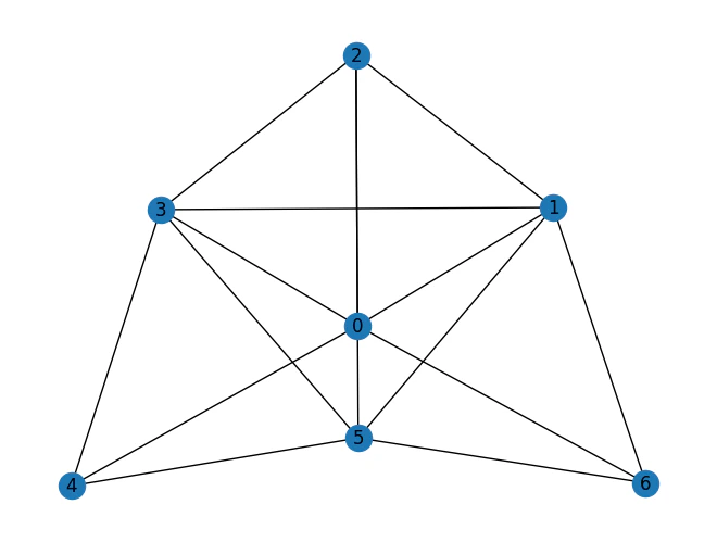
This tutorial solves the max clique problem in graph theory using Classiq.A clique is a subset of vertices in a graph such that each pair is adjacent to one other.Given a graph G=(V,E), find the maximal clique in the graph. It is known to be in the NP-hard complexity class.
import networkx as nximport numpy as npimport pyomo.environ as pyodef define_max_clique_model(graph): model = pyo.ConcreteModel() # each x_i states if node i belongs to the cliques model.x = pyo.Var(graph.nodes, domain=pyo.Binary) x_variables = np.array(list(model.x.values())) # define the complement adjacency matrix as the matrix where 1 exists for each non-existing edge adjacency_matrix = nx.convert_matrix.to_numpy_array(graph, nonedge=0) complement_adjacency_matrix = ( 1 - nx.convert_matrix.to_numpy_array(graph, nonedge=0) - np.identity(len(model.x)) ) # constraint that 2 nodes without edge in the graph cannot be chosen together model.clique_constraint = pyo.Constraint( expr=x_variables @ complement_adjacency_matrix @ x_variables == 0 ) # maximize the number of nodes in the chosen clique model.value = pyo.Objective(expr=sum(x_variables), sense=pyo.maximize) return model
To solve the Pyomo model defined above, use the CombinatorialProblem Python class.Under the hood, it translates the Pyomo model to a quantum model of the Quantum Approximate Optimization Algorithm (QAOA) [1], with a cost Hamiltonian translated from the Pyomo model.Choose the number of layers for the QAOA ansatz using the num_layers argument:
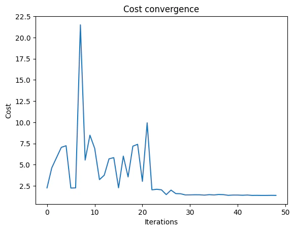
Solve the problem by calling the optimize method of the CombinatorialProblem object.For the classical optimization part of the QAOA algorithm, define the maximum number of classical iterations (maxiter) and the α-parameter (quantile) for running CVaR-QAOA, an improved variation of the QAOA algorithm [2]:
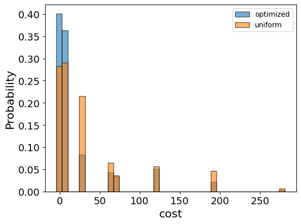
Examine the statistics of the algorithm.The optimization is always defined as a minimization problem, so the Pyomo-to-Qmod translator changes the positive maximization objective to negative minimization.To get samples with the optimized parameters, call the sample method:
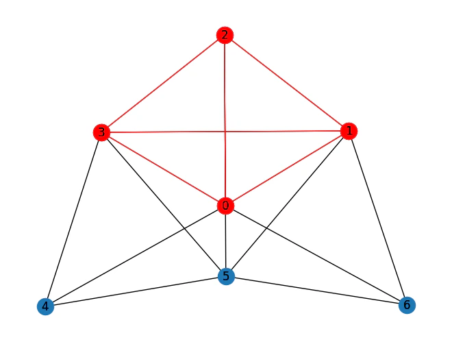
solution_nodes = [v for v in graph.nodes if best_solution["x"][v]]solution_edges = [ (u, v) for u, v in graph.edges if u in solution_nodes and v in solution_nodes]nx.draw_kamada_kawai(graph, with_labels=True)nx.draw_kamada_kawai( graph, with_labels=True, nodelist=solution_nodes, edgelist=solution_edges, node_color="r", edge_color="r",)
Lastly, compare to the classical solution of the problem:
from pyomo.opt import SolverFactorysolver = SolverFactory("couenne")solver.solve(max_clique_model)classical_solution = [ int(pyo.value(max_clique_model.x[i])) for i in range(len(max_clique_model.x))]print("Classical solution:", classical_solution)
Output:
Classical solution: [1, 1, 1, 1, 0, 0, 0]
solution = [int(pyo.value(max_clique_model.x[i])) for i in graph.nodes]solution_nodes = [v for v in graph.nodes if solution[v]]solution_edges = [ (u, v) for u, v in graph.edges if u in solution_nodes and v in solution_nodes]nx.draw_kamada_kawai(graph, with_labels=True)nx.draw_kamada_kawai( graph, with_labels=True, nodelist=solution_nodes, edgelist=solution_edges, node_color="r", edge_color="r",)