Use this file to discover all available pages before exploring further.
View on GitHub
Open this notebook in GitHub to run it yourself
The quantum counting algorithm [1] efficiently estimates the number of valid solutions to a search problem, based on the amplitude estimation algorithm. It demonstrates a quadratic improvement with regard to a classical algorithm with black box oracle access to the function f.More precisely, given a Boolean function f:{0,1}n→{0,1}, the counting problem estimates the number of inputs x to f such that f(x)=1.This tutorial demonstrates how to estimate the counting problem using a specific variant of the amplitude estimation algorithm: the Iterative Quantum Amplitude Estimation (IQAE) [2].The IQAE does not rely on the Quantum Phase Estimation algorithm [3], but purely on applications of the grover operator:Q≡−AS0A†Sψ1,thereby reducing the required number of qubits and gates of the circuit, at the expense of additional multiplicative factor polylogarithmic in the error ϵ.
We choose this equation:(a+b)<=2where a, b are 2-bit unsigned integers.This equation has six solutions.The goal is to estimate the number of valid solutions out of the 16 possible inputs, with precision 0.5.
We first show how to use quantum phase estimation algorithm for quantum counting [3], then solve it using the IQAE method.Given a state ∣ψ⟩ such that ∣ψ⟩=a∣ψ1⟩+1−a∣ψ0⟩ we can measure a up to arbitrary precision, given the following building blocks:
State preparation:
A unitary A such that: A∣0⟩=∣ψ⟩=a∣ψ1⟩+1−a∣ψ0⟩.
Oracle:
A unitary Sψ1 such that Sψ1=I−2∣ψ1⟩⟨ψ1∣, which adds a (−1) phase to ∣ψ1∣ψ⟩⟩ and does nothing to any orthognal states to ∣ψ1⟩.
This is effectively a reflection around the “good” state ∣ψ1⟩.Given these two functions, we can construct the Grover operator:Q≡−AS0A†Sψ1,which is exactly the same operator as for the Grover’s search algorithm.In the subspace spanned by ∣ψ1⟩ and ∣ψ0⟩, Q has two eigenvalues:λ±=exp(±i2πθ),sin2(πθ)≡a.Therefore, if we apply a QPE on A∣0⟩ we have these two eigenvalues encoded in the QPE register; however, both give the value of a, so there is no ambiguity.
The state preparation function A reflects knowledge about the solution space and can be used to eliminate invalid assignments.Here we assume no knowledge of the solution space; hence, we use the uniform superposition state preparation.
We use the grover_operator library function, where we plug in the defined oracles. We wrap it by the qpe function, that accepts the grover operator as a unitary, and additional phase register.
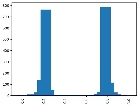
Upon plotting the resulting histogram, we see two phase values with high probability (however, both correspond to the same amplitude).Note that phase_reg is already coded as fixed QNum in the range [0,1].
import matplotlib.pyplot as pltphases_counts = dict( (sampled_state.state["phase_reg"], sampled_state.shots) for sampled_state in result.parsed_counts)plt.bar(phases_counts.keys(), phases_counts.values(), width=0.1)plt.xticks(rotation=90)print("phase with max probability: ", max(phases_counts, key=phases_counts.get))
Output:
phase with max probability: 0.78125
From the phase, we can extract the number of solutions:
Amplitude Estimation Using Iterative Quantum Amplitude Estimation
Now we are ready for the iterative method.Instead of QPE, the algorithm applies the unitary(Q)mAwhere m, the number of repetitions, changes between iterations of the algorithm.There is one subtlety that changes the way we work with the Grover operator.The classical algorithm expects an additional indicator qubit that marks the “good” states, i.e.:∣a⟩∣b⟩∣f(a,b)⟩So now, most of our logic goes into the state preparation oracle (A). It combines the loading of the solution space with setting the indicator qubit.
Wrapping All to the Iterative Quantum Amplitude Estimation Algorithm
We use the built-in IQAE class that the quantum code for the algorithm as well as the classical execution code.The circuit starts with the state A∣0⟩, then applies iterations of the Grover operator.Note that the algorithm applies a varied number of Grover iterations on each execution.The number of iterations is chosen dynamically based on previous execution results, using statistical inference methods. It expects a state preparation function that creates the following state:∣Ψ⟩=a∣Ψ1⟩∣1⟩ind+1−a2∣Ψ0⟩∣0⟩indWhere the indicator qubit is marking the wanted state.
from classiq.applications.iqae.iqae import IQAEiqae = IQAE( state_prep_op=iqae_state_preparation, problem_vars_size=DOMAIN_SIZE, constraints=Constraints(optimization_parameter="width"), preferences=Preferences(optimization_level=1),)
We can also see the statistics of the IQAE execution:
for i, iteration in enumerate(iqae_result.iterations_data):
    print(
        f"iteration_id: {i}, num grover iterations: {iteration.grover_iterations}, counts: {iteration.sample_results.counts}"
    )