Optimize - The Synthesis Engine

View on GitHub Experiment in the IDE

The previous section focused on how to design quantum algorithms with the Qmod language. Once you have designed a quantum algorithm, the Classiq synthesis engine compiles it into a quantum circuit ready for implementation on quantum computers or simulators. This section covers how to use the Classiq synthesis engine in the IDE and the Python SDK through concrete examples.

Synthesis Background

In most cases, a specific quantum model can be compiled to many or sometimes an infinite number of quantum circuits that might differ in their properties. Some may have more qubits with smaller circuit depth, some may have all the qubits connected to each other whilst others do not, and some may have fewer 2-qubit gates than others.

The Classiq synthesis engine receives the quantum model as input together with the constraints and preferences of the desired quantum program, and outputs a quantum program implementation of the quantum model that satisfies the constraints and preferences.

Some of the available constraint options for the synthesis engine: * Optimization parameter - either to optimize for circuit width or circuit depth; * Maximal gate count - maximum allowed number of a specific 1- or 2-qubit gate; * Maximal circuit width or circuit depth.

Some of the available preferences: * Compiling the quantum circuit for a specific quantum processor; * The desired connectivity map of the quantum circuit; * The output format of the quantum circuit, e.g., QASM or QIR.

See a full list of constraints and preferences in the reference manual.

This section covers how to apply constraints and preferences through an actual example.

Concrete Example

The task covered in the 'Design - The Qmod Language' tutorial is to create a quantum algorithm that calculates the arithmetic expression \(y=x^2+1\) in a superposition.

The following model written in Qmod implements the desired task:

PythonNative

from classiq import *


@qfunc
def main(x: Output[QNum], y: Output[QNum]):

    allocate(4, x)
    hadamard_transform(x)  # creates a uniform superposition
    y |= x**2 + 1

qfunc main(output x: qnum, output y: qnum) {
  allocate<4>(x);
  hadamard_transform(x);
  y = (x ** 2) + 1;
}

You can always directly synthesize it without any constraints or preferences:

quantum_program = synthesize(create_model(main))

Now, apply constraints and preferences; first in the IDE, and then in the Python SDK.

Constraints and Preferences in the IDE

In the IDE, once your model is complete, you can directly synthesize your algorithm with the default constraints and preferences by clicking Synthesize:

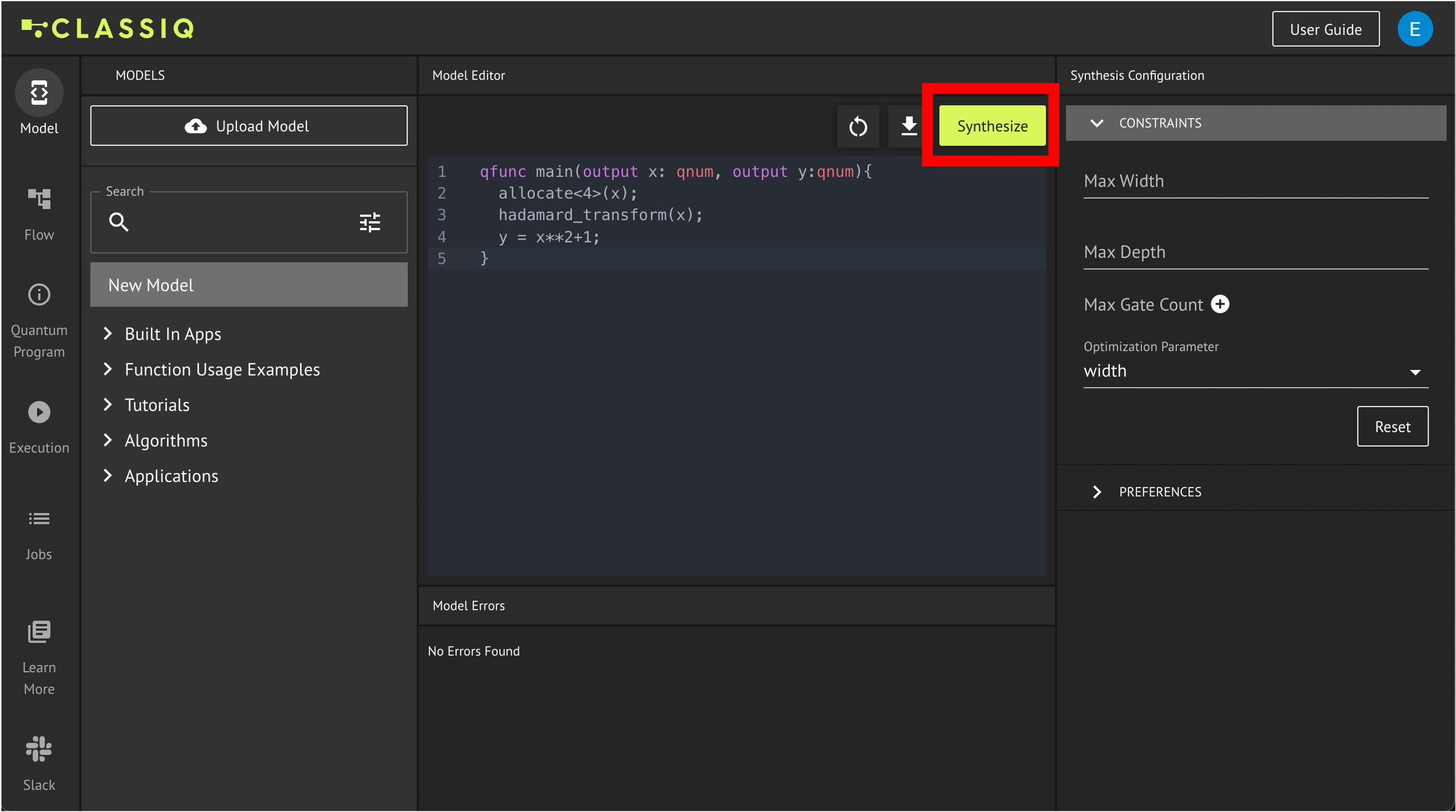
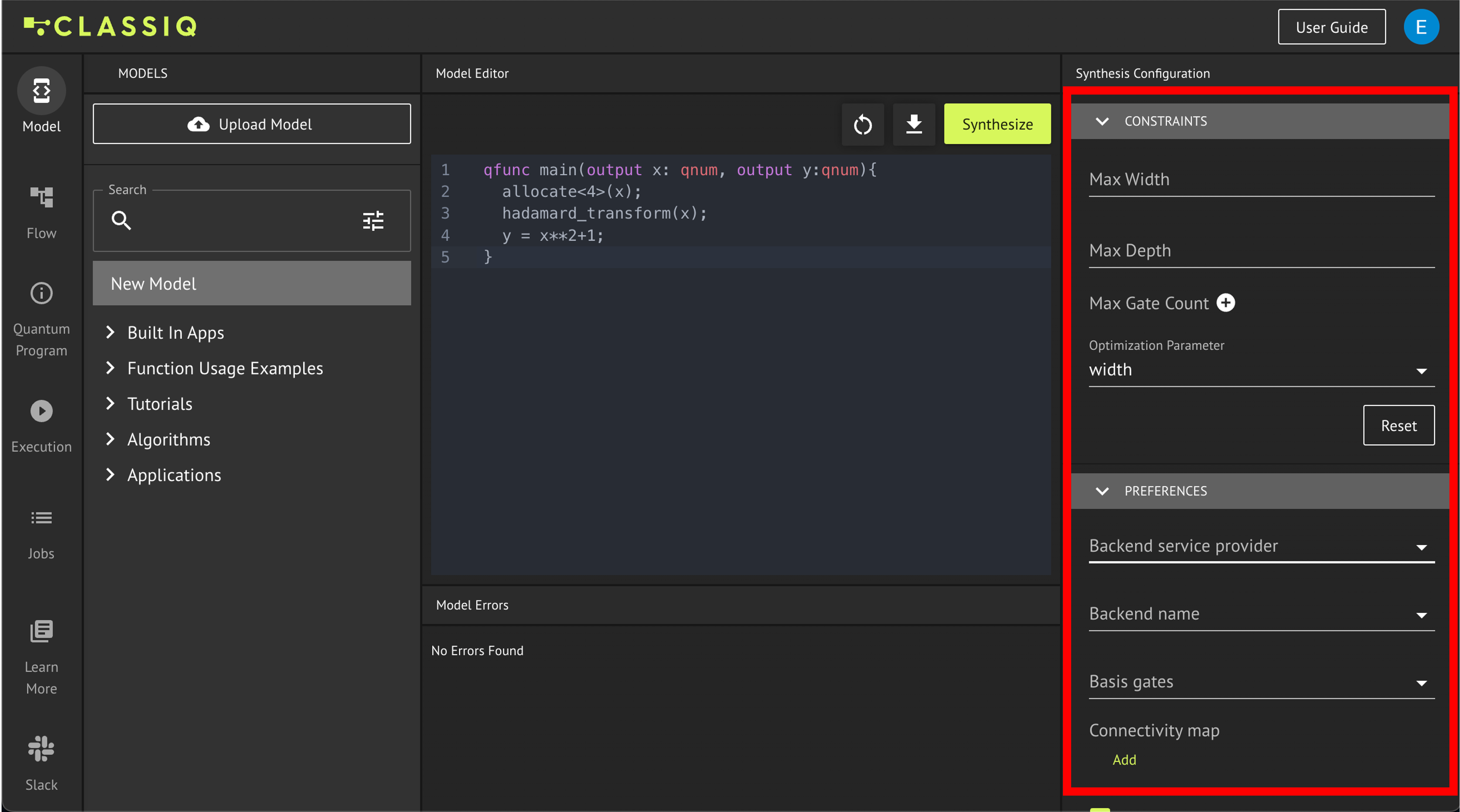
To apply constraints and preferences, adapt the parameters on the right of the window and then synthesize your model:

Below, see how to configure the constraints and preferences in the Python SDK.

Constraints and Preferences in the Python SDK

The synthesis engine receives an underlying Qmod representation of the quantum model that you construct in the Python SDK using the create_model function:

quantum_model = create_model(main)

You can synthesize this quantum_model directly with the command synthesize(quantum_model) to return the quantum program implementation. However, to apply constraints and preferences, first adapt the quantum_model representation.

Create a circuit with the minimum number of qubits and a maximum circuit depth of \(500\) by applying these constraints to the quantum_model:

quantum_model_with_constraints = set_constraints(
    quantum_model, Constraints(optimization_parameter="width", max_depth=500)
)

Synthesize the quantum_model as usual:

quantum_program = synthesize(quantum_model_with_constraints)

Extract the parameters of the circuit implementation:

circuit_width = QuantumProgram.from_qprog(quantum_program).data.width
circuit_depth = QuantumProgram.from_qprog(quantum_program).transpiled_circuit.depth
print(f"The circuit width is {circuit_width} and the circuit_depth is {circuit_depth}")

Compilation versus Transpilation

The synthesis engine is a compiler that compiles a high-level functional model to one specific circuit out of many possible implementations. A transpiler, on the other hand, transforms one circuit implementation to another. Its use can be to change from a circuit representation with a given basis gate set to another one, or to further optimize a given circuit implementation with basic optimization procedures such as cancellation of two identical Hermitian gates applied consequently.

It is highly recommended that you complete the following exercise yourself, to experience for the first time how the one quantum algorithm can be compiled into two different circuit implementations that can substantially differ from one other.

Recommended Exercise

Modify the constraints above to optimize the circuit for minimum circuit depth using maximum 25 qubits. What circuit depth and width do you receive? Are they different than shown above? Analyze the two quantum circuits using `show(quantum_program)` and determine which functional building block is implemented differently.

For the purpose of the exercise, assume that you will execute the quantum model on the ibm_brisbane IBM quantum processor. Pass this information to the synthesis engine so the quantum program is built appropriately. Do it by adding this preference and resynthesizing quantum_model:

quantum_model_with_preferences = set_preferences(
    quantum_model,
    Preferences(backend_service_provider="IBM Quantum", backend_name="ibm_brisbane"),
)

quantum_program = synthesize(quantum_model_with_preferences)

Optional Exercise

Extract the circuit depth and width of the above quantum program. How do they differ from the previous values? Consider why they differ in such a way. (It is helpful to know that the `IBM Brisbane` device has specific limited connectivity between its qubits, so there might be a certain overhead in applying some 2-qubit gates.)

So now you have a quantum program that implements the quantum model that calculates \(y=x^2+1\) in a superposition, optimized for a specific real quantum computer. The following sections show how to actually run it on that computer with Classiq. But first, dive deeply into the Classiq analysis capabilities.

Verify Your Understanding - Recommended Exercise

Synthesize 3 different implementations of an MCX (multi-control-x) with 5 control qubits and 1 target qubit (you should use the control quantum operation for implementing an MCX, follow this tutorial that can be open in the IDE). One implementation should be optimized for minimized depth, the other for minimized width, and the third somewhere in between (choose yourself what is the maximal width / depth you apply).

Export the 3 implementations as LaTeX files on the hierarchy level that demonstrates the differences between the implementations. Aggregate the implementations in 1 file and export it as a PDF and explain the key differences (it is recommended to use Overleaf - a free, easy to use online LaTeX editor).

Advanced Exercise

Synthesize 5 different implementations of an MCX with 20 control qubits and 1 target qubit. Compare the circuit width and circuit depth required for each implementation.

write_qmod(quantum_model_with_constraints, "optimize")