Binary Knapsack
Background
Given a set of items, determine how many items to put in the knapsack to maximize their summed value.
Define:
-
\(x_i\) is the number of items from each type.
-
\(v_i\) is the value of each item.
-
\(w_i\) is the weight of each item.
-
\(D\) is the range of \(x\).
Find \(x\) that maximizes the value: \(\begin{aligned} \max_{x_i \in D} \Sigma_i v_i x_i\\ \end{aligned}\)
and constrained by the weight: \(\begin{aligned} \Sigma_i w_i x_i = C \end{aligned}\)
Problem Versions
Binary Knapsack
Range: \(D = \{0, 1\}\)
Integer Knapsack
Range: \(D = [0, b]\)
Knapsack with binary variables and equality constraint
Define the optimization problem
import numpy as np
import pyomo.environ as pyo


def define_knapsack_model(weights, values, max_weight):
    model = pyo.ConcreteModel()
    num_items = len(weights)

    model.x = pyo.Var(range(num_items), domain=pyo.Binary)

    x_variables = np.array(list(model.x.values()))

    model.weight_constraint = pyo.Constraint(expr=x_variables @ weights == max_weight)

    model.value = pyo.Objective(expr=x_variables @ values, sense=pyo.maximize)

    return model
Initialize the model with parameters
knapsack_model = define_knapsack_model(
    weights=[2, 3, 2.1, 1, 1, 2], values=[3, 5, 2, 1.5, 1.2, 2.7], max_weight=5
)
Setting Up the Classiq Problem Instance
In order to solve the Pyomo model defined above, we use the Classiq combinatorial optimization engine. For the quantum part of the QAOA algorithm (QAOAConfig) - define the number of repetitions (num_layers):
from classiq import construct_combinatorial_optimization_model
from classiq.applications.combinatorial_optimization import OptimizerConfig, QAOAConfig

qaoa_config = QAOAConfig(num_layers=5)
For the classical optimization part of the QAOA algorithm we define the maximum number of classical iterations (max_iteration) and the \(\alpha\)-parameter (alpha_cvar) for running CVaR-QAOA, an improved variation of the QAOA algorithm [3]:
optimizer_config = OptimizerConfig(max_iteration=60, alpha_cvar=0.7)
Lastly, we load the model, based on the problem and algorithm parameters, which we can use to solve the problem:
qmod = construct_combinatorial_optimization_model(
    pyo_model=knapsack_model,
    qaoa_config=qaoa_config,
    optimizer_config=optimizer_config,
)
We also set the quantum backend we want to execute on:
from classiq import set_execution_preferences
from classiq.execution import ClassiqBackendPreferences, ExecutionPreferences

backend_preferences = ExecutionPreferences(
    backend_preferences=ClassiqBackendPreferences(backend_name="simulator")
)

qmod = set_execution_preferences(qmod, backend_preferences)
from classiq import write_qmod

write_qmod(qmod, "knapsack_binary")
Synthesizing the QAOA Circuit and Solving the Problem
We can now synthesize and view the QAOA circuit (ansatz) used to solve the optimization problem:
from classiq import show, synthesize

qprog = synthesize(qmod)
show(qprog)
Opening: https://platform.classiq.io/circuit/db610424-2d79-4db4-8c6c-17734c34b003?version=0.41.0.dev39%2B79c8fd0855
We now solve the problem by calling the execute function on the quantum program we have generated:
from classiq import execute

res = execute(qprog).result()
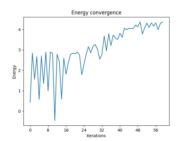
We can check the convergence of the run:
from classiq.execution import VQESolverResult

vqe_result = res[0].value
vqe_result.convergence_graph
Optimization Results
We can also examine the statistics of the algorithm:
import pandas as pd

from classiq.applications.combinatorial_optimization import (
    get_optimization_solution_from_pyo,
)

solution = get_optimization_solution_from_pyo(
    knapsack_model, vqe_result=vqe_result, penalty_energy=qaoa_config.penalty_energy
)
optimization_result = pd.DataFrame.from_records(solution)
optimization_result.sort_values(by="cost", ascending=False).head(5)
| probability | cost | solution | count | |
|---|---|---|---|---|
| 62 | 0.003 | 8.0 | [1, 1, 0, 0, 0, 0] | 3 |
| 24 | 0.017 | 7.7 | [0, 1, 0, 1, 1, 0] | 17 |
| 59 | 0.007 | 7.7 | [0, 1, 0, 0, 0, 1] | 7 |
| 2 | 0.028 | 7.5 | [1, 1, 0, 1, 0, 0] | 28 |
| 11 | 0.024 | 7.2 | [0, 1, 0, 1, 0, 1] | 24 |
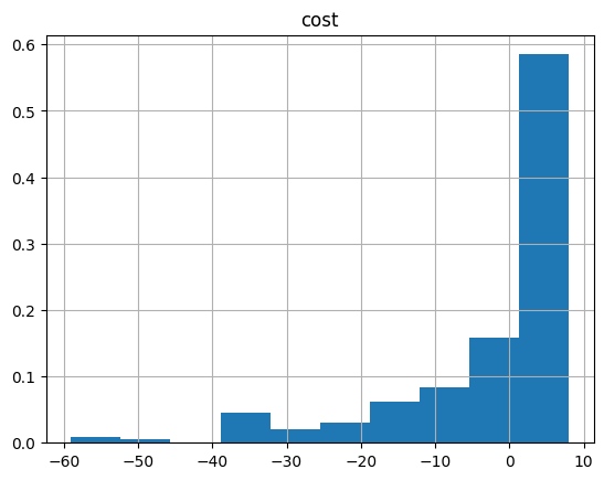
And the histogram:
optimization_result.hist("cost", weights=optimization_result["probability"])
array([[<Axes: title={'center': 'cost'}>]], dtype=object)
Lastly, we can compare to the classical solution of the problem:
from pyomo.opt import SolverFactory

solver = SolverFactory("couenne")
solver.solve(knapsack_model)

knapsack_model.display()
Model unknown

  Variables:
    x : Size=6, Index=x_index
        Key : Lower : Value                 : Upper : Fixed : Stale : Domain
          0 :     0 :    0.9999999999999998 :     1 : False : False : Binary
          1 :     0 :                   1.0 :     1 : False : False : Binary
          2 :     0 :                   0.0 :     1 : False : False : Binary
          3 :     0 :                   0.0 :     1 : False : False : Binary
          4 :     0 :                   0.0 :     1 : False : False : Binary
          5 :     0 : 2.220446049250313e-16 :     1 : False : False : Binary

  Objectives:
    value : Size=1, Index=None, Active=True
        Key  : Active : Value
        None :   True :   8.0

  Constraints:
    weight_constraint : Size=1
        Key  : Lower : Body : Upper
        None :   5.0 :  5.0 :   5.0