

- Studio Python: code in Python directly in the browser. No local installation required.
- Local Python SDK: code in Python from your local environment, notebook, or preferred editor.
- Qmod in the Classiq Platform: write Qmod directly in the browser-based Model Editor.
To use Classiq, you need a Classiq account. Register through the Classiq Platform or follow the registration guide.
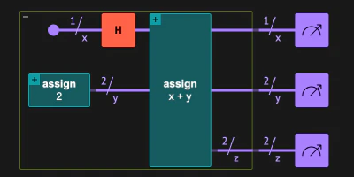
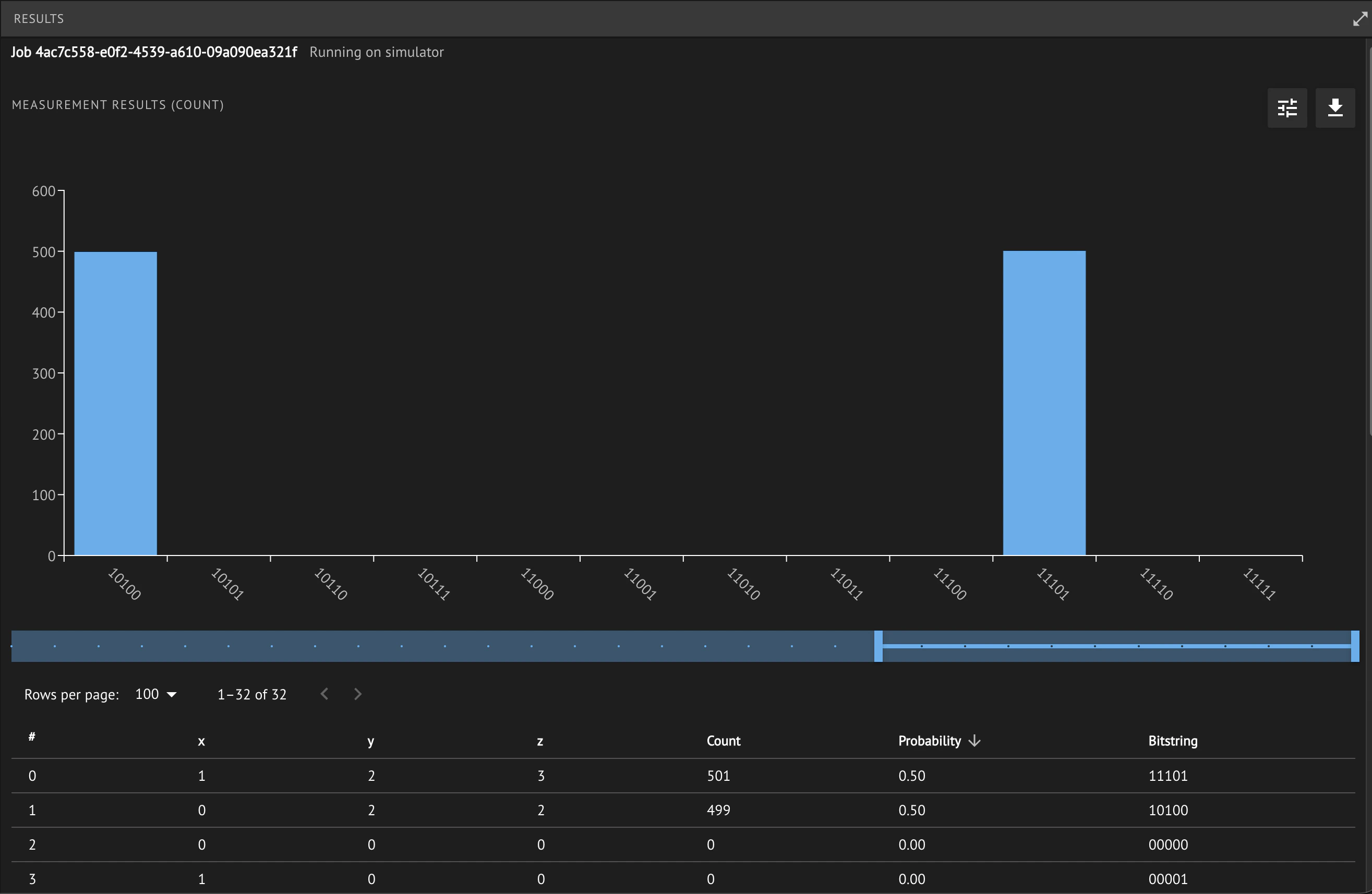
x: a one-qubit quantum number prepared in superposition.y: a quantum number assigned the value2.z: a quantum number that stores the expressionx + y.
x is placed in superposition, execution samples two possible arithmetic outcomes:
- When
x = 0,z = 2. - When
x = 1,z = 3.
- Created a simple Qmod model
- Synthesized it into a quantum program
- Executed it
- Verified that the results show the expected relation between
x,y, andz
- Use Python in Classiq Studio if you want to work with Python in a setup-free, cloud-based coding editor.
- Use the Python SDK locally if you want to work in notebooks or scripts in your local development environment.
- Use Qmod-native syntax in the Classiq Platform if you want to write Qmod directly in the browser-based Model Editor.
- Studio Python SDK
- Local Python SDK
- Classiq Platform
Use the Classiq Studio if you want to build, synthesize, execute, and inspect quantum programs directly in your browser while still coding in Python -
no need to install anything.Open the Classiq Studio and create the arithmetic model in a new file: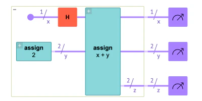
x, and an arithmetic block is applied between
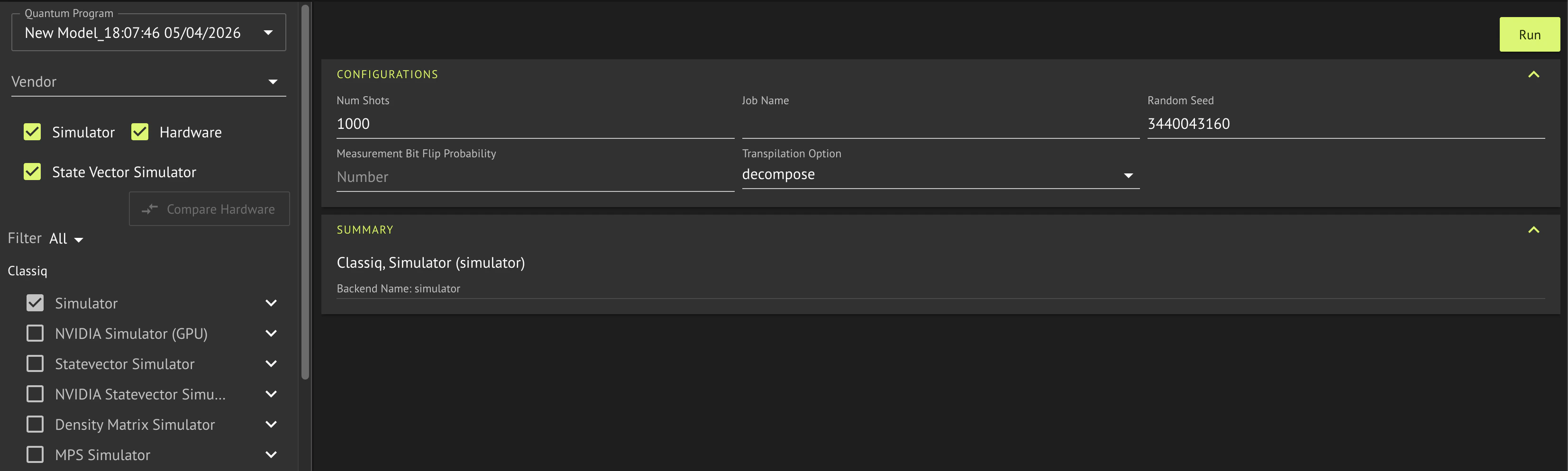
x, y, and z to perform the equation .To execute the quantum program, run:Your exact counts may differ, but the measured results should contain only and , with roughly equal probabilities.
This is the result of the arithmetic operation executed by the quantum program.In this path, you used
synthesize to compile the high-level model into a quantum program, show to visualize it, and sample to execute it and inspect the measurement results.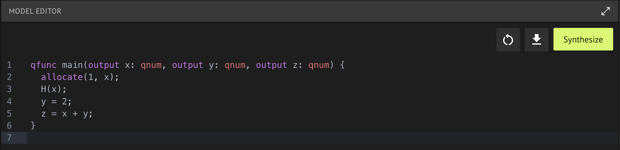
What this example introduced
This first program introduced the main ideas you will use throughout Classiq:- A quantum function defines reusable quantum logic.
mainis the entry point of a Qmod model.allocateinitializes quantum variables.- Quantum gates such as
Hthat manipulates quantum information. - Synthesis compiles a high-level model into a quantum program.
- Execution runs the quantum program and returns measurement results.
- Result analysis helps you verify that the program behaves as expected.
Next steps
Choose your next tutorial based on your goal:- Learn Qmod fundamentals: Qmod Tutorial, Part 1
- Go deeper into Qmod: Qmod Tutorial, Part 2
- Understand synthesis and optimization: Synthesis Tutorial
- Learn execution workflows: Execution Tutorial, Part 1
- Work with parameterized and variational workflows: Execution Tutorial, Part 2