

View on GitHub
Open this notebook in GitHub to run it yourself
Combinatorial Optimization Workshop using the Qmod quantum types - part 1
In this workshop, we will solve the MaxCut problem using qmod’s quantum types, such asQBit, and the phase function. First, we will have introduction to the Maximum Cut (MaxCut) problem.
Guidance for the workshop:
The# TODO is there for you to do yourself.
**The # Solution start and # Solution end are only for helping you.
Please delete the Solution and try doing it yourself…**
Introduction
The “Maximum Cut Problem” (MaxCut) [1] is an example of combinatorial optimization problem. It refers to finding a partition of a graph into two sets, such that the number of edges between the two sets is maximal. This optimization problem is the cardinal example in the context of Quantum Approximate Optimization Algorithm [2], since it is an unconstrained problem whose objective function in terms quantum gates can be derived easily. With the Classiq platform, things are even simpler, as the objective function is inserted in its arithmetic form.Mathematical formulation
Given a graph with nodes and edges, a cut is defined as a partition of the graph into two complementary subsets of nodes. In the MaxCut problem we are looking for a cut where the number of edges between the two subsets is maximal. We can represent a cut of the graph by a binary vector of size , where we assign 0 and 1 to nodes in the first and second subsets, respectively. The number of connecting edges for a given cut is simply given by summing over for every pair of connected nodes .Solving with the Classiq platform
We go through the steps of solving the problem with the Classiq platform, using QAOA algorithm [2].Creating and plotting the graph, the MaxCut problem
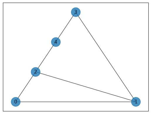
Create the classical optimization function
First, build a function that whether to count an edge or not. If the two nodes are from different groups, the functionedge_cut will return 1, otherwise, it should return
- The values of the nodes are binary.
Generic building blocks for QAOA circuit
The mixer layer will applyRX gates with parameter beta to all qubits in the qba array.
The phase function
In the QAOA ansatz, the cost layer gives a phase to any solution type. Therefore, we will use thephase function which takes an expression (phase_expr) and a parameter (coefficient) as arguments.
See more here.
For example:
phase function rotates each computational basis state about the Z axis with the angle coefficient relative the value of the expression phase_expr. Namely, it adds a phase to each quantum state with respect to the value that returns.
The quantum variables constitute the quantum state .
Problem specifc building blocks
Synthesizing and visualizing
Output:
Execution and post processing
For the hybrid execution, we useExecutionSession, which can evaluate the circuit in multiple methods, such as sampling the circuit, giving specific values for the parameters, and evaluating to a specific Hamiltonian, which is very common in chemical applications.
In QAOA, we will use the estimate_cost method, which samples the cost function and returns their average cost from all measurements.
That helps to optimize easily.
- This approach showed better solutions because it is similar to the adiabatic evolution with big steps rather than small evolution.
ExecutionSession to calculate the cost of all measurements at once using the estimate_cost method.
estimate_cost method give the .
But you can define anything with the estimate_cost, not necessarily the expectation value of the Hamiltonian.
Define the callback function to store the intermediate parameters or any intermediate parameter you wish.
minimize function from scipy.
You need to combine the objective function, which includes the quantum program, the classical optimizer, and the callback function.
To achieve better convergence, you need to define the type of optimizer (such as COBYLA), the number of iterations, and other parameters, depending on the type of optimizer.
maxiter is the number of iterations. As the number of layers is larger, we need more iterations to converge to a good solution because there are more parameters.
After we finish the optimization and find good parameters, we will use them once again to find the optimized solution.
Output:
Plot the result
Let’s plot the result of the best found solution.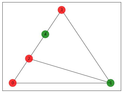
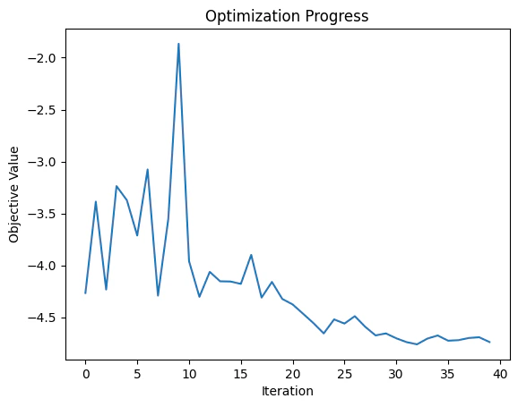
Plot the convergence graph
Changes to play with
- Change the type of the optimizer from the scipy minimize function.
- Each optimizer has another type step size.
rhobeg.
The step size determines how far the optimizer will go in each iteration.
You can change it to see how it affects the convergence.
- Do the same optimization process for a random Erdos Renyi graph.
- Build a weighted graph in which each edge has a different weight, and solve the maxcut with it.