High-Level Algorithm Design with Qmod Part II

View on GitHub

Open this notebook in GitHub to run it yourself

QAOA Knapsack

In Part I we looked at specific high-level language concepts, their meaning and use. In this part, we apply these concepts to design a full algorithm. We will consider alternative ways to implement the Quantum Approximate Optimization Algorithm (QAOA). In particular, we will compare two approaches to expressing the hard constraint of the knapsack problem - using a penalty term in phase rotations and using a digital (computational-basis) conditional. The goal of the exercise is to demonstrate the use of quantum expressions in different modes, and their combination. It is not meant as a comprehensive study of hard constraints in QAOA, nor does it consider many other factors that determine QAOA performance and results (a rich and active field of research). There are 3 code exercises in this notebook with the corresponding heading and a code snippet containing TODO comments. Make sure to complete the code in the snippets before running the cell. Solutions are provided at the end of the notebook. Don’t continue to the next exercise until you have completed the previous one and compared against the solution.

Warm-Up: QAOA Pattern in Qmod (Max-Cut Example)

We start by reviewing a simple demonstration of the QAOA algorithm. It solves a trivial case of the max-cut problem (but can easily be generalized to arbitrary graphs). The purpose of this code is just to get acquainted with the Qmod implementation, and define a couple of the building blocks that we shall reuse later.

from classiq import *

NUM_LAYERS = 3


# Python function encapsulating the cost expression (reused in ansatz and classical optimizer loop)
def maxcut_cost(v: QArray[QBit, 3]):  # Toy graph with 3 nodes and 2 edges
    graph_edges = [(0, 1), (0, 2)]
    return -sum(v[n1] ^ v[n2] for (n1, n2) in graph_edges)


@qfunc
def cost_layer(v: QArray[QBit], gamma: CReal):
    phase(maxcut_cost(v), gamma)


@qfunc
def init_layer(v: QArray[QBit]):
    apply_to_all(lambda q: H(q), v)


@qfunc
def mixer_layer(v: QArray[QBit], beta: CReal):
    apply_to_all(lambda q: RX(beta, q), v)


@qfunc
def main(
    params: CArray[CReal, NUM_LAYERS * 2],
    v: Output[QArray[QBit, 3]],
):
    gammas = params[0:NUM_LAYERS]
    betas = params[NUM_LAYERS : 2 * NUM_LAYERS]
    allocate(v)
    init_layer(v)
    for i in range(NUM_LAYERS):
        cost_layer(v, gammas[i])
        mixer_layer(v, betas[i])


qprog = synthesize(main)
show(qprog)

Output:

Quantum program link: https://platform.classiq.io/circuit/3IjJPqZgLmiHFRhFE6kgLV9GxQQ
  

Output:

https://platform.classiq.io/circuit/3IjJPqZgLmiHFRhFE6kgLV9GxQQ?login=True&version=22
  

To execute the algorithm we use the ExecutionSession.variational_minimize method which uses gradient descent to optimize the parameters of the ansatz. The cost function is defined as the expectation value of the cost operator, which is defined in the maxcut_cost function above. The initial parameters are set to a linear schedule, which is a common heuristic for QAOA.

import numpy as np

# Start with a linear scheduling guess
INIT_GAMMAS = [0, np.pi / 2, np.pi]
INIT_BETAS = [np.pi, np.pi / 2, 0]
initial_params = INIT_GAMMAS + INIT_BETAS

with ExecutionSession(qprog) as es:
    trace = es.variational_minimize(
        cost_function=lambda v: maxcut_cost(v),
        initial_params={"params": initial_params},
        max_iteration=40,
    )
    df = es.sample(parameters=trace[-1][1]).dataframe
    display(df)

	v	counts	probability	bitstring
0	[1, 0, 0]	956	0.466797	001
1	[0, 1, 1]	927	0.452637	110
2	[1, 1, 0]	42	0.020508	011
3	[1, 0, 1]	39	0.019043	101
4	[0, 1, 0]	37	0.018066	010
5	[0, 0, 1]	29	0.014160	100
6	[0, 0, 0]	12	0.005859	000
7	[1, 1, 1]	6	0.002930	111

The optimal solution to this trivial max-cut problem is the partition into node sets {0} and {1, 2}.

The QAOA cost layer for graph problems can be expressed directly in Qmod using phase statement with a bitwise expression.

The Knapsack Problem

The general definition of the knapsack problem is the following: Given a set of items, determine how many items to put in the knapsack to maximize their summed value.

Input:
Item count of each kind $x_i$ , where $x_i \in [0, d_i]$ .
Item weights, denoted as $w_i$ .
Item values, denoted as $v_i$ .
Weight constraint $C$ .
Output:
Item assignment $\overline{x}$ that maximizes the value: $\max_{x_i \in D} \Sigma_i v_i x_i$ subject to a weight constraint: $\Sigma_i w_i x_i\leq C$ .
The feasible value for a given assignment is the value sum if the constraint is satisfied and otherwise zero.

The knapsack is known to be an NP-complete problem. Here we choose a small toy instance:

2 item types:
- $a \in [0, 7]$ with $w_a=2$ , $v_a=3$
- $b \in [0, 3]$ with $w_b=3$ , $v_b=5$
$C=12$

The optimal solution for the problem is (spoiler alert!)

a=3, b=2

Exercise 1: Modeling the Knapsack Problem

In this exercise we will model the knapsack problem in Qmod.

Use quantum numeric variables as fields of a quantum struct to represent the item counts.
Use quantum expressions to represent the value and weight, as well as the constraint.

class KnapsackVars(QStruct):
    # TODO: Modify the declaration of problem variables 'a' and 'b' to the appropriate quantum type
    a: QBit
    b: QBit


def value_sum(v: KnapsackVars):
    # TODO: Return the value sum expression
    return 0  # Remove this line (placeholder to avoid syntax error)


def weight_sum(v: KnapsackVars):
    # TODO: Return the weight sum expression
    return 0  # Remove this line (placeholder to avoid syntax error)


def constraint(v: KnapsackVars):
    # TODO: Use weight_sum() to return the Boolean constraint expression
    return 0  # Remove this line (placeholder to avoid syntax error)


def feasible_value(v: KnapsackVars):
    return value_sum(v) if constraint(v) else 0


# A little hack to test our conditions..
class dotdict(dict):
    __getattr__ = dict.get


print(feasible_value(dotdict(a=3, b=2)))
print(feasible_value(dotdict(a=3, b=3)))

Output:

0
  0
  

The assignment a=3 and b=2 is the optimal solution for our toy model with value 19, but any violation of the constraint is value

Having defined the variables using Qmod types, the problem can be captured directly in Qmod expressions.

Execution Utility Function

You can skip this section if you are not interested in the details of the execution flow we shall subsequently use. They are not important for our exercise. With the above general problem description we can define a helper function that optimizes the anasatz parameters for our knapsack problem and displays the results. The flow is not different from the example we saw above. , but note that we optimize on a function that reflects a linear gradiant for both the knapsack value and the violation of the constraint. Based on the optimized parameters, we sample the ansatz and calculate the probability of samples that satisfy the constraint, the average value of the feasible samples, and the overall value average. We will compare the different ansatz structures, keeping all other parameters fixed, and specifically using the same logic to obtain these results.

from matplotlib import pyplot as plt

from classiq.qmod.symbolic import max as qmod_max


def optimize_qaoa_params(ansatz, max_iteration):
    with ExecutionSession(ansatz) as es:
        # Optimize the parameters to minimize cost function value
        def opt_cost_function(v):
            return -value_sum(v) + 4 * qmod_max(weight_sum(v) - 12, 0)

        opt_trace = es.variational_minimize(
            cost_function=opt_cost_function,
            initial_params={"params": initial_params},
            max_iteration=max_iteration,
        )
        final_params = opt_trace[-1][1]
        cost_trace = [c[0] for c in opt_trace]

        # Plot the cost convergence
        plt.plot(cost_trace)
        plt.xlabel("Iterations")
        plt.ylabel("Cost")
        plt.title("Cost convergence")
        plt.show()

        print_statistics(es.sample(parameters=final_params))
        return final_params


def print_statistics(res):
    feas = [s for s in res.parsed_counts if constraint(s.state["v"])]
    feas_shots = sum(s.shots for s in feas)
    val_sum = sum(value_sum(s.state["v"]) * s.shots for s in feas)
    avg_val_sum = sum(feasible_value(s.state["v"]) * s.shots for s in res.parsed_counts)
    print(f"Probability of feasible solution: {feas_shots / res.num_shots:.4f}")
    print(f"Average feasible values: {val_sum / feas_shots if feas_shots else 0:.4f}")
    print(f"Overall score: {avg_val_sum / res.num_shots:.4f}")


def sample_anzatz(anzatz, params, num_shots):
    df = sample(anzatz, parameters=params, num_shots=num_shots)
    df["feasible value"] = df.apply(
        lambda row: feasible_value(dotdict(a=row["v.a"], b=row["v.b"])), axis=1
    )
    return df

Representing Hard Constraints as Cost

The cost operator in QAOA is typically defined in terms of QUBO expressions, or more generally low-degree polynomials over problem variables. In Qmod this is directly expressible using the phase statement. But logical operators are not allowed in the phase expression, because they cannot be reduced to low-degree polynomials. The feasible value defined by the problem is the value sum if the constraint is satisfied and otherwise zero. An expression of this form cannot be used directly in phase statement. A common approach is to add to the overall cost a penalty term for violating the constraint. For equality constraints we can square the difference between the variable expression and its target to obtain a non-negative penalty. However, in the knapsack case we need to represent an inequality constraint. An inequality expression can be rewritten as an equality by introducing a non-negative slack (“don’t-care”) variable that represents the difference between the left and right sides of the inequality. When evaluating an assignment the slack variable is disregarded. As an example, the constraint

x + y \leq 10

can be expressed as

x + y + slack = 10

. In this case the penalty will be

(x + y + slack - 10)^2

. The cost layer multiplies the penalty term can be given more significance by multiplying it by a constant “penalty factor”, e.g.

2*(x + y + slack - 10)^2

. The penalty approach has the downside of not representing the true semantics of the problem. It incentivises assignments that have high value with only a small violation of the constraint. But our problem is defined in terms of a hard constraint, where even a small violation means zero actual value. In Exercise 2 we will define the cost operator in terms of the constraint penalty term, and in Exercise 3 we will define it to accurately capture the Boolean condition.

Exercise 2: The Knapsack Constraint as a Penalty Term

In this exercise we will implement the knapsack problem using a penalty term to represent the constraint.

Use the fields of struct KnapsackVarsPenalty to express the penalty term.
Define the cost layer in terms of the value sum and the penalty term.
Execute the algorithm and observe the results:
What is the probability of a feasible sample? What is the average value of the feasible samples?
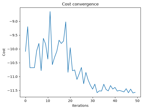
How many iterations did it take to converge to a solution?

class KnapsackVarsPenalty(QStruct):
    a: QNum[3]
    b: QNum[2]
    slack: QNum[4]


def constraint_slack_penalty(v):
    # TODO: Return the slack penalty expression
    pass  # Remove this line (placeholder to avoid syntax error)


@qfunc
def cost_layer(v: KnapsackVarsPenalty, gamma: CReal):
    # TODO: Define the cost phase shift in terms of value_sum() and constraint_slack_penalty()
    pass


@qfunc
def main(
    params: CArray[CReal, NUM_LAYERS * 2],
    v: Output[KnapsackVarsPenalty],
):
    allocate(v)
    init_layer(v)
    for i in range(NUM_LAYERS):
        cost_layer(v, params[i])
        mixer_layer(v, params[NUM_LAYERS + i])


qprog = synthesize(main)
show(qprog)
final_params = optimize_qaoa_params(qprog, max_iteration=50)
df = sample_anzatz(qprog, params=final_params, num_shots=10)
display(df)

Output:

Quantum program link: https://platform.classiq.io/circuit/3IjJSs709B6RQn68dkcq8gH05By
  

Output:

https://platform.classiq.io/circuit/3IjJSs709B6RQn68dkcq8gH05By?login=True&version=22
  

Output:


Submitting job to simulator

Output:

Probability of feasible solution: 0.0000
  Average feasible values: 0.0000
  Overall score: 0.0000
  

Output:


Job: https://platform.classiq.io/jobs/f3deeaab-ba64-44ae-b57b-8fa1e75ad2cb

	v.a	v.b	v.slack	counts	probability	bitstring
0	7	2	3	1	0.1	001110111
1	6	2	6	1	0.1	011010110
2	2	0	7	1	0.1	011100010
3	4	3	7	1	0.1	011111100
4	4	0	10	1	0.1	101000100
5	6	3	11	1	0.1	101111110
6	7	1	12	1	0.1	110001111
7	3	0	13	1	0.1	110100011
8	0	2	13	1	0.1	110110000
9	7	3	15	1	0.1	111111111

The overall score is the expectation value of assignments, computed on a large sample.The table shows a small sample from the same distribution, with assignments and their value.Value 0 typically means a violation of the constraint.

The cost function, including the penalty for the violation of an inequality constraint can be expressed in Qmod directly as a second degree polynomial.

Exercise 3: The Knapsack Constraint as a Boolean Condition

In this exercise we will implement the knapsack problem using a Boolean condition to represent the constraint.

Use the fields of struct KnapsackVars (from Exercise 1) to express the cost layer as a phase shift for the value sum, conditioned on the constraint.
Look at the quantum program visualization and note the structure of the cost layer.

Compare the implementation of the two expression forms.

Execute the algorithm and inspect the results:
How does the probability of a feasible sample and the average value compare to the penalty-term approach?
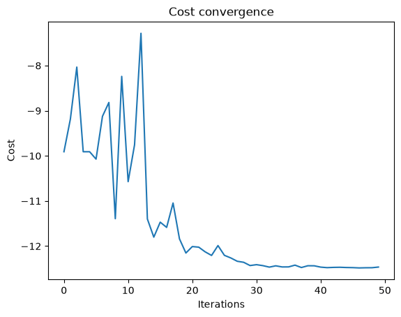
How many iterations did it take to converge to a solution with this ansatz structure?

@qfunc
def cost_layer(v: KnapsackVars, gamma: CReal):
    # TODO: Define the cost as phase shift by value_sum(), under the condition that the constraint is satisfied
    pass


@qfunc
def main(
    params: CArray[CReal, NUM_LAYERS * 2],
    v: Output[KnapsackVars],
):
    allocate(v)
    init_layer(v)
    for i in range(NUM_LAYERS):
        cost_layer(v, params[i])
        mixer_layer(v, params[NUM_LAYERS + i])


qprog = synthesize(main)
show(qprog)
final_params = optimize_qaoa_params(qprog, max_iteration=50)
df = sample_anzatz(qprog, params=final_params, num_shots=10)
display(df)

Output:

Quantum program link: https://platform.classiq.io/circuit/3IjJWT9PEk9PVJ5Wwzp7SbCiAbd
  

Output:

https://platform.classiq.io/circuit/3IjJWT9PEk9PVJ5Wwzp7SbCiAbd?login=True&version=22
  

Output:

Probability of feasible solution: 0.0000
  Average feasible values: 0.0000
  Overall score: 0.0000
  

Output:


Submitting job to simulator

Output:


Job: https://platform.classiq.io/jobs/2befba64-3c0f-452b-8457-908147be53d5

	v.a	v.b	counts	probability	bitstring
0	1	0	4	0.4	01
1	0	1	3	0.3	10
2	0	0	2	0.2	00
3	1	1	1	0.1	11

The optimizer converges with fewer iterations using the more accurate ansatz, compared to the one in Exercise 2.The expectation value of the distribution is often also improved, but this varies and is sensitive to the random decisions of the optimizer.

The QAOA cost layer in Qmod can comprise computational-basis conditions and polynomial evaluation in the phase, which together represent the true semantics of the problem.Note that phase oracle in Grover search (as shown in Part I, Exercise 5) can be seen as a special case of such a QAOA cost layer, with only a Boolean condition and no phase preference between the “good” states.

Solutions

Solution to Exercise 1

class KnapsackVars(QStruct, dict):
    # Declare the problem variables 'a' and 'b' as quantum numeric variables
    a: QNum[3]
    b: QNum[2]


def value_sum(v: KnapsackVars):
    # Return the value expression
    return v.a * 3 + v.b * 5


def weight_sum(v: KnapsackVars):
    # Return the total weight expression
    return v.a * 2 + v.b * 3


def constraint(v: KnapsackVars):
    # Use weight_sum() to return the Boolean constraint expression
    return weight_sum(v) <= 12


def feasible_value(v: KnapsackVars):
    return value_sum(v) if constraint(v) else 0


class dotdict(dict):
    __getattr__ = dict.get


print(feasible_value(dotdict(a=3, b=2)))
print(feasible_value(dotdict(a=3, b=3)))

Output:

19
  0
  

Solution to Exercise 2

class KnapsackVarsPenalty(QStruct):
    a: QNum[3]
    b: QNum[2]
    slack: QNum[4]


PENALTY_FACTOR = 2


def constraint_slack_penalty(v):
    # Return the slack penalty expression
    return PENALTY_FACTOR * (weight_sum(v) + v.slack - 12) ** 2


@qfunc
def cost_layer(v: KnapsackVarsPenalty, gamma: CReal):
    # Define the cost phase shift using value_sum and constraint_slack_penalty
    phase(-value_sum(v) + constraint_slack_penalty(v), gamma)


@qfunc
def main(
    params: CArray[CReal, NUM_LAYERS * 2],
    v: Output[KnapsackVarsPenalty],
):
    allocate(v)
    init_layer(v)
    for i in range(NUM_LAYERS):
        cost_layer(v, params[i])
        mixer_layer(v, params[NUM_LAYERS + i])


qprog = synthesize(main)
# show(qprog)
final_params = optimize_qaoa_params(qprog, max_iteration=50)
df = sample_anzatz(qprog, params=final_params, num_shots=10)
display(df)

Output:

Probability of feasible solution: 0.5952
  Average feasible values: 13.1698
  Overall score: 7.8389
  

Output:


Submitting job to simulator

Output:


Job: https://platform.classiq.io/jobs/2ece5bae-a8af-4e51-a2dc-b407e848b418

	v.a	v.b	v.slack	counts	probability	bitstring	feasible value
0	6	1	11	2	0.2	101101110	0
1	1	1	0	1	0.1	000001001	8
2	5	3	1	1	0.1	000111101	0
3	3	2	6	1	0.1	011010011	19
4	4	2	6	1	0.1	011010100	0
5	4	3	7	1	0.1	011111100	0
6	6	0	9	1	0.1	100100110	18
7	7	1	9	1	0.1	100101111	0
8	1	2	10	1	0.1	101010001	13

Solution to Exercise 3

@qfunc
def cost_layer(v: KnapsackVars, gamma: CReal):
    # Define the cost as phase shift by value_sum(), under the condition that the constraint is satisfied
    control(constraint(v), lambda: phase(-value_sum(v), gamma))


@qfunc
def main(
    params: CArray[CReal, NUM_LAYERS * 2],
    v: Output[KnapsackVars],
):
    allocate(v)
    init_layer(v)
    for i in range(NUM_LAYERS):
        cost_layer(v, params[i])
        mixer_layer(v, params[NUM_LAYERS + i])


qprog = synthesize(main)
# show(qprog)
qprog = synthesize(main)
final_params = optimize_qaoa_params(qprog, max_iteration=50)
df = sample_anzatz(qprog, params=final_params, num_shots=10)
display(df)

Output:

Probability of feasible solution: 0.5610
  Average feasible values: 14.0592
  Overall score: 7.8877
  

Output:


Submitting job to simulator

Output:


Job: https://platform.classiq.io/jobs/76ac414c-971a-46b0-b908-d2f632a6fb67

	v.a	v.b	counts	probability	bitstring	feasible value
0	5	1	3	0.3	01101	0
1	2	3	2	0.2	11010	0
2	0	1	1	0.1	01000	5
3	0	3	1	0.1	11000	15
4	1	3	1	0.1	11001	18
5	3	3	1	0.1	11011	0
6	7	3	1	0.1	11111	0

Algorithms

Applications

Tutorials

High-Level Algorithm Design with Qmod Part II

View on GitHub

QAOA Knapsack

Warm-Up: QAOA Pattern in Qmod (Max-Cut Example)

The Knapsack Problem

Exercise 1: Modeling the Knapsack Problem

Execution Utility Function

Representing Hard Constraints as Cost

Exercise 2: The Knapsack Constraint as a Penalty Term

Exercise 3: The Knapsack Constraint as a Boolean Condition

Solutions

Solution to Exercise 1

Solution to Exercise 2

Solution to Exercise 3

View on GitHub

​QAOA Knapsack

​Warm-Up: QAOA Pattern in Qmod (Max-Cut Example)

​The Knapsack Problem

​Exercise 1: Modeling the Knapsack Problem

​Execution Utility Function

​Representing Hard Constraints as Cost

​Exercise 2: The Knapsack Constraint as a Penalty Term

​Exercise 3: The Knapsack Constraint as a Boolean Condition

​Solutions

​

​Solution to Exercise 1

​

​Solution to Exercise 2

​

​Solution to Exercise 3

QAOA Knapsack

Warm-Up: QAOA Pattern in Qmod (Max-Cut Example)

The Knapsack Problem

Exercise 1: Modeling the Knapsack Problem

Execution Utility Function

Representing Hard Constraints as Cost

Exercise 2: The Knapsack Constraint as a Penalty Term

Exercise 3: The Knapsack Constraint as a Boolean Condition

Solutions

Solution to Exercise 1

Solution to Exercise 2

Solution to Exercise 3