

View on GitHub
Open this notebook in GitHub to run it yourself
Option Pricing
An option is the possibility to buy (call) or sell (put) an item (or share) at a known price (the strike price, K), where the option has a maturity price (S). For example, this is the payoff function to describe a European call option: $f(S)=\Bigg{\begin{array}{lr} 0, & \text{when } K\geq S\ S
- K, & \text{when } K < S\end{array} $
- Load the distribution, i.e., discretize the distribution using points (where n is the number of qubits) and truncate it.
- Implement the payoff function that is equal to zero if and increases linearly otherwise.
- Evaluate the expected payoff using amplitude estimation.
Designing The Quantum Algorithm
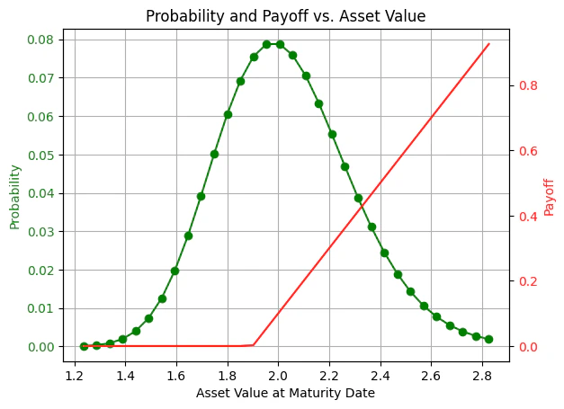
Probability Distribution
The distribution describes the option underlying asset price at maturity date. Load a discrete version of the log normal probability with points, when is equal tomu, is equal to sigma, and is equal to num_qubits.
In addition, choose K, the strike price:
Output:
Output:
Quantum Function for the Distribution Loading
The generalinplace_prepare_state function is needed as it is repeatedly applied on the same quantum variable.
For simplicity, use the general purpose state preparation.
There are more efficient and scalable methods for preparing the required distribution; for example, see [4].
Payoff Function
Create the payoff function by loading . When building the European call option function, do nothing if the strike price is smaller than ; otherwise, apply a linear amplitude loading. NOTE: To save qubits and depth, the register holds a value in the range , “labeling” the asset value. The mapping to the asset value space occurs in the comparator and amplitude loading, using this (classical)scale function:
assign_amplitude_table function.
The calculation is exact, however it is not scalable for large variable sizes.
More scalable methods are mentioned in [4] and [6].
Important: So that all loaded amplitudes are not greater than 1, normalize the payoff by a scaling_factor, later multiplied in the post-process stage:
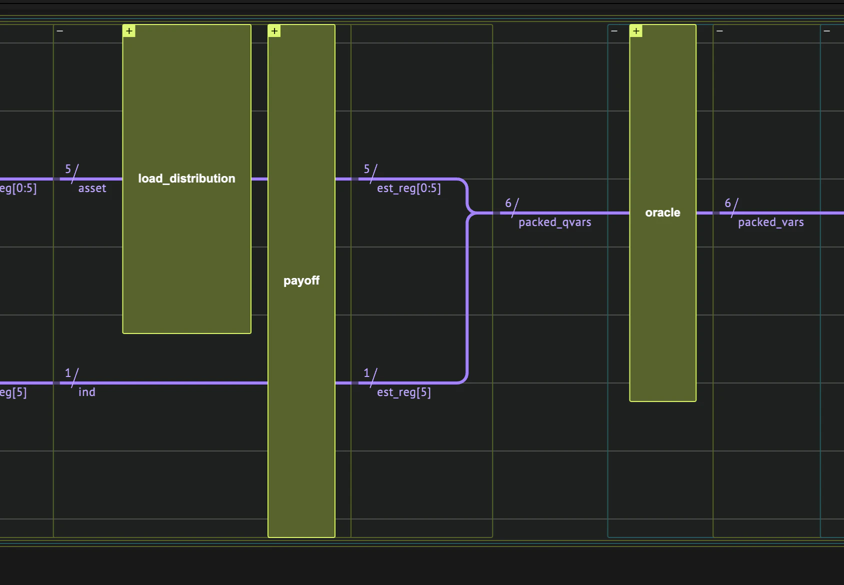
Wrapping to an Amplitude Estimation Model
After defining the probability distribution and the payoff function, pack them together as a state preparation in the Iterative Quantum Amplitude Estimation algorithm [5]. The oracle is very simple and only needs to recognize whether the indicator qubit is in the state. The returned amplitude from the algorithm is according to the formula: which approximates the expectation value of the payoff: The built-inIQAE application expects a state preparation operand, and builds a model for the iterative amplitude estimation algorithm:
Quantum Program Synthesis
Synthesize the model to a quantum program:Output:
Quantum Program Execution
Define the parameters for the accuracy of the amplitude estimation. This affects the expected number of Grover of repetitions within the execution:scaling_factor:
Output:
Output: