

View on GitHub
Open this notebook in GitHub to run it yourself
- Using the VQE Primitive
- Using the PyTorch Integration
- Using the QSVM Built-in App
In This Tutorial
- Using the VQE Primitive
- Using the PyTorch Integration
- Using QSVM Primitive
Using the VQE Primitive
The Variational Quantum Eigensolver (VQE) is an algorithm for finding the ground state energy of a Hamiltonian operator, often described by Pauli operators or in the equivalent matrix form. The VQE was proposed in 2014 [1]. The algorithm follows these steps:- Create a Parameterized Quantum Model: Design a quantum model, also known as an ansatz, that captures the problem.
- Synthesize, Execute, and Estimate Expectation Values: Synthesize the quantum model into a quantum program.
- Optimize Parameters: Use a classical optimizer to adjust the quantum program’s parameters for better results.
- Repeat: Continue this process until the algorithm converges to a solution or reaches a specified number of iterations.
Example Using Classiq
Start with this example, creating a VQE algorithm that estimates the minimal eigenvalue of the following 2x2 Hamiltonian: Define the Hamiltonian usingPauli terms:
NOTE on U-gate
NOTE on U-gate
The single-qubit gate applies phase and rotation with three Euler angles.Matrix representation:Parameters:
-
theta:CReal -
phi:CReal -
lam:CReal -
gam:CReal -
target:QBit
main, and use the minimize attribute from ExecutionSession to optimize it.
Description of ExecutionSession Minimize Parameters
Description of ExecutionSession Minimize Parameters
Configure the
minimize function in the ExecutionSession workflow with these parameters:- cost_function: The cost function to minimize, it can be either a quantum a quantum cost function specified by a Hamiltonian or a classical function that is represented as a callable and returns a Qmod expression.
- initial_params: Initial parameters for the optimization routine. It accepts only a single parameter and should be formatted as a dict in the form {“parameter”: list}.
- max_iteration: The maximum number of iterations for the optimizer.
- quantile: The quantile-based cutoff for which outcomes to consider when estimating the cost function.
float values of the cost function and its respective parameters.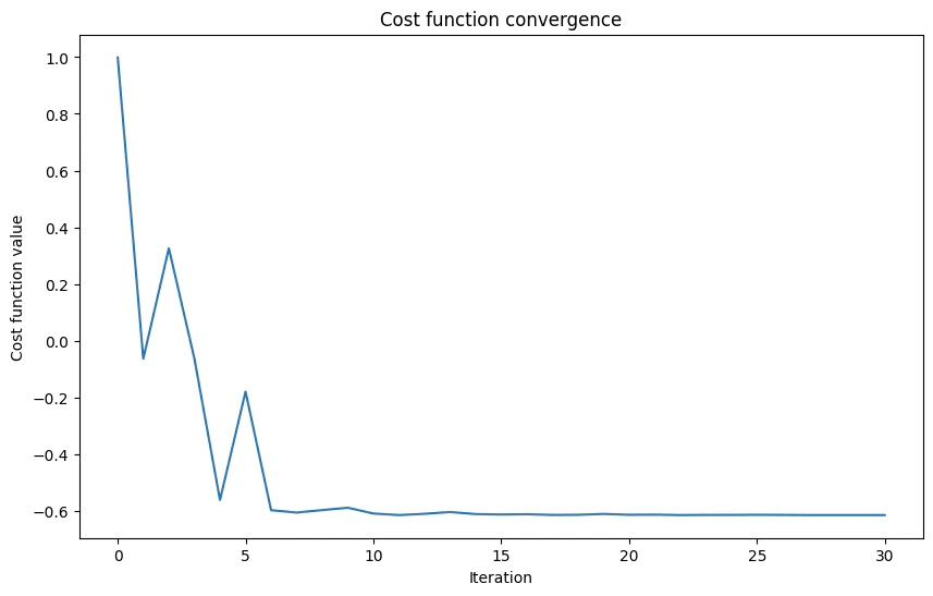
Output:
- Optimal energy: The lowest energy found for the Hamiltonian, representing the ground state energy (minimal eigenvalue).
- Optimal parameters: The parameters of the quantum program that achieve the optimal energy, corresponding to rotation angles in the U-gate.
- Eigenstate: The quantum state associated with the optimal energy, given as probability amplitudes for the basis states.
Summary and Exercise
You designed a parameterized quantum circuit capable of capturing a simple Hamiltonian. You initialized anExecutionSession and used minimize to execute it, visualizing the results.
Exercise
- Two Qubits VQE
Exercise - Two Qubits VQE
Now, practice the implementation of a similar case to the previous example, but this time for two qubits, following the Hamiltonian:Use the last example to implement and execute VQE for this Hamiltonian.Code skeleton:
Read More
Further reading from the reference manual:Using the PyTorch Integration
Classiq integrates with PyTorch, enabling the seamless development of quantum machine learning and hybrid classical quantum machine learning models. This integration leverages PyTorch’s powerful machine learning capabilities alongside quantum computing.Note on PyTorch Installation:
Note on PyTorch Installation:
To properly install and run PyTorch locally, check this page.
Workflow
- Defining the Model
- 1.1: Define the quantum model and synthesize it into a quantum program.
- 1.2: Define the execute and post-process callables.
-
1.3: Create a
torch.nn.Modulenetwork.
- Choosing the Dataset, Loss Function, and Optimizer
- Training the Model
- Testing the Model
PyTorch Documentation
PyTorch Documentation
Example
This example demonstrates PyTorch integration using a simple parameterized quantum model. It utilizes one input from the user and one weight, while using one qubit in the model. The goal of the learning process is to determine the correct angle for an RX gate to perform a “NOT” operation. (Spoiler alert: The correct answer is .) The datasetDATALOADER_NOT is used, as defined here.
DatasetXor is also available from the link for further practice.
Output:
0.0000) and is labeled as 0, indicating the state .
The second item indicates a rotation of 3.1416 and is labeled as 1, indicating the state .
Read an explanation on creating PyTorch datasets here:
Step 1.1
- Define the Quantum Model and Synthesize It into a Quantum Program
mixing function, which includes an adjustable parameter for training the RX gate to act later as a NOT gate:
main function:
Output:
Step 1.2
- Define the Execute and Postprocess Callables
execute and post-processing functions.
These functions are essential for integrating the quantum layer in a PyTorch neural network, as classical layers require classical data as input.
This means that only after executing the QLayer (the ansatz) and post-processing the results the data can be further used in other layers of the neural network or be output.
The execute function is straightforward. It takes the quantum program (here, the QLayer) and its parameters, and executes it:
Output:
post_process function is needed to prepare the execution results for output or for loss calculation during the training phase.
In this specific example, it returns the probability of measuring .
This function assumes that only the differentiation between the single state and all other states is relevant. If a different differentiation is needed, modify this function accordingly.
Step 1.3
- Create a torch.nn.Module Network
torch.nn.Module class with a single QLayer as follows:
self.qlayer = QLayer(...), define the only layer in the neural network as a single QLayer.
Specify the previously defined quantum_program, execute, and post_process as arguments for the layer. Finally, create the neural network and assign it to the variable model.
Step 2
- Choose a Dataset, Loss Function, and Optimizer
Available Optimization Algorithms and Loss Functions
Available Optimization Algorithms and Loss Functions
For details of the optimization algorithms and a comprehensive list of loss functions in PyTorch, refer to the official documentation:
Step 3
ImportDataLoader:
DataLoader in PyTorch efficiently iterates over datasets, handling batching, shuffling, and parallel data loading. It streamlines the process of training and evaluating models by managing data efficiently.
Now you are ready to define the training function. This simple example follows a loop similar to that recommended by PyTorch here.
You may comment on the following cell, change the number of epochs above, and expect about 40 epochs for full training for non-trained parameters.
Output:
Now, test the network accuracy using the suggested method here.
Output:
Output:
model.qlayer.weight, which is a tensor of shape (1,1).
After training, this value should be close to .
Summary and Exercise
In this tutorial, you integrated a quantum layer in a PyTorch neural network, defined the necessary execution and post-processing functions, and trained the model using a simple dataset. You tested the network’s accuracy using a recommended method. To explore further, try experimenting with different quantum circuits, datasets, and optimizers. Integrating more classic layers or more complex layers should be straightforward now for those with experience in PyTorch.Exercise
- Training U Gate
Exercise - Training U Gate
Now, for practice, implement a similar case to the last example, but this time train the U gate to act as a NOT gate instead of the Rx gate.
How many parameters must you train?
What must you change to accomplish this?
How many parameters must you train?
What must you change to accomplish this?
Hint
Hint
You only have to adapt
mixing and model.