

View on GitHub
Open this notebook in GitHub to run it yourself
Introduction
The set cover problem [1] represents a well-known problem in the fields of combinatorics, computer science, and complexity theory. It is an NP-complete problems. The problem presents us with a universal set, , and a collection of subsets of . The goal is to find the smallest possible subfamily, , whose union equals the universal set. Formally, let’s consider a universal set and a collection containing subsets of , with . The challenge of the set cover problem is to find a subset of of minimal size such that .Solving with the Classiq platform
We go through the steps of solving the problem with the Classiq platform, using QAOA algorithm [2]. The solution is based on defining a pyomo model for the optimization problem we would like to solve.Building the Pyomo model from an input
We proceed by defining the pyomo model that will be used on the Classiq platform, using the mathematical formulation defined above:- Binary variable for each subset (model.x) indicating if it is included in the sub-collection.
- Objective rule – the size of the sub-collection.
- Constraint – the sub-collection covers the original set.
Output:
Setting Up the Classiq Problem Instance
In order to solve the Pyomo model defined above, we use theCombinatorialProblem quantum object.
Under the hood it tranlastes the Pyomo model to a quantum model of the QAOA algorithm, with a cost function translated from the Pyomo model. We can choose the number of layers for the QAOA ansatz using the argument num_layers, and the penalty_factor, which will be the coefficient of the constraints term in the cost hamiltonian.
Synthesizing the QAOA Circuit and Solving the Problem
We can now synthesize and view the QAOA circuit (ansatz) used to solve the optimization problem:Output:
Output:
optimize method of the CombinatorialProblem object.
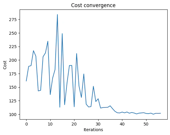
For the classical optimization part of the QAOA algorithm we define the maximum number of classical iterations (maxiter) and the -parameter (quantile) for running CVaR-QAOA, an improved variation of the QAOA algorithm [3]:
Output:
Optimization Results
We can also examine the statistics of the algorithm. In order to get samples with the optimized parameters, we call thesample method:
| solution | probability | cost | |
|---|---|---|---|
| 52 | {‘x’: [0, 1, 0, 1, 1, 0, 0, 0], ‘independent_r… | 0.001465 | 23.0 |
| 66 | {‘x’: [0, 1, 0, 1, 1, 0, 0, 0], ‘independent_r… | 0.001465 | 23.0 |
| 1107 | {‘x’: [0, 1, 0, 0, 1, 0, 1, 0], ‘independent_r… | 0.000488 | 23.0 |
| 636 | {‘x’: [1, 0, 1, 1, 0, 0, 0, 0], ‘independent_r… | 0.000488 | 23.0 |
| 1531 | {‘x’: [0, 1, 0, 0, 1, 0, 1, 0], ‘independent_r… | 0.000488 | 23.0 |
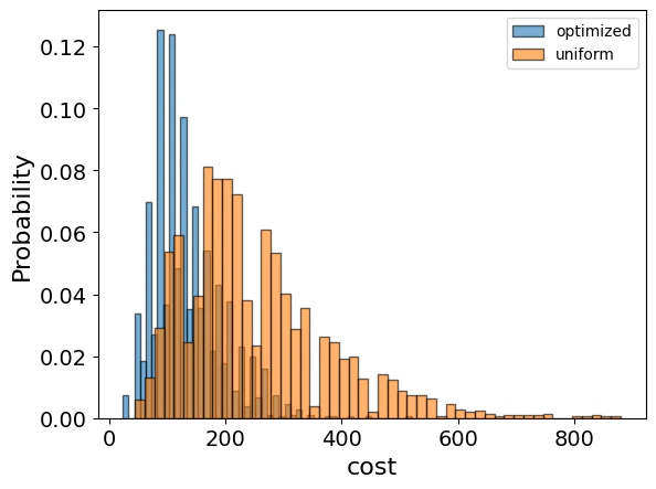
Output:
Output:
Comparison to a classical solver
Lastly, we can compare to the classical solution of the problem:Output:
Output: