View on GitHub
Open this notebook in GitHub to run it yourself
Currently, more than 100,000 patients are on the waiting list in the United States for a kidney transplant from a deceased donor. This is addressed by a program called the Kidney Exchange Program. This program won the 2012 Nobel Prize in Economics for Alvin E. Roth and Lloyd S. Shapley’s contributions to the theory of stable matchings and the design of markets. In summary, in a donor pair, the recipient needs a kidney transplant and a donor is willing to give a kidney to the recipient. About of those pairs are not compatible for a direct exchange. This is tackled by considering two incompatible pairs together: Donor 1 may be compatible with Recipient 2, and Donor 2 may be compatible with Recipient
- In this example, a two-way swap becomes feasible.
Creating a Pyomo Model for a Simple Kidney Exchange Problem
In this very simple example, patients and donors represent sets of patients who receive a kidney from a donor. Compatibility is a dictionary mapping of patient-donor pairs to their compatibility scores. Binary decision variables are defined for each patient-donor pairx[donor,patient].
The objective is to maximize the total compatibility score:
where
- d=donors
- p=patients
- c=compatability score
Output:
Generating the QAOA Process
Creating Parameters for the Quantum Circuit
Create the initial parameters, modifying them when necessary:- Define the number of layers (
num_layers) of the QAOA ansatz. - Define
penalty_energyfor invalid solutions, which influences the convergence rate.
Forming the QAOA Model as a Qmod
Combine everything together to form the entire QAOA model as a Qmod:- Synthesize the quantum model.
- Show the quantum model in the Classiq platform.
Output:
Output:
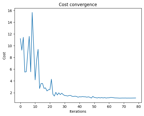
Defining the Classical Optimizer Part of the QAOA
Modify these parameters:max_iterations- maximum number of optimizer iterations, set to
quantile- describes the quantile considered in the CVaR expectation value.
NOTE: When looking at the graph, recall that this is a maximization problem.
Output:
Retrieving and Displaying the Solutions
To view the solutions:- Print them out
- Graph them using a histogram
- Show `Donor
- Recipients` in Network Graph
Print Best Solutions
Print out the top 10 solutions with the highest cost or objective:Output:
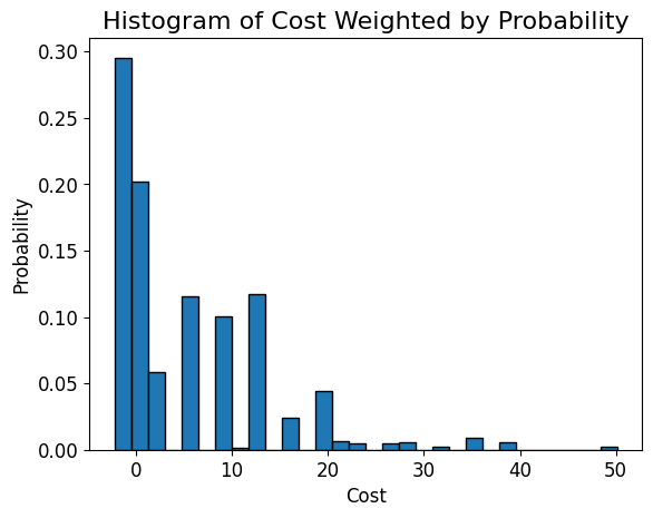
Histogram of Cost, Weighted by Probability
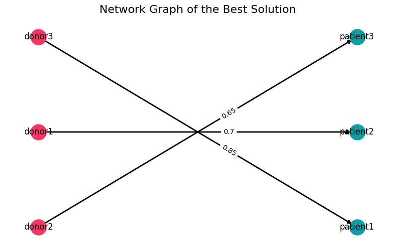
Creating a Network Graph
Create a network graph for the best solution found. NOTE: This is a maximization problem and the classical solver of the QAOA process returns all possible results. Filter out the solution with the highest cost that represents the the highest compatability score:Output: