

View on GitHub
Open this notebook in GitHub to run it yourself
- One to one compares classical random walks with quantum walks via a specific example: a walk on a circle.
- A general quantum model studies quantum walks and subsequently applies it to the circle case and to a hypercube graph.
- The resemblance between classical and quantum programming with Classiq.
- Classiq’s built-in constructs:
-
control: general controlled-logic -
power: “parametric power”, specified as execution parameter. -
numeric quantum types: working with signed and unsigned integers. -
within_apply: for compute/uncompute operations . -
Passing a list of
QCallables(quantum functions). - Parsed execution results, according to quantum variable types.
Classical Random Walks Versus Quantum Walks
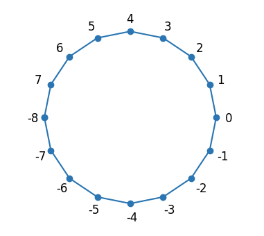
Specify and implement a simple example: a discrete walk on a circle, or more precisely, on a regular polygon with nodes (see Figure 1). The idea behind the random/quantum walk:- Start at some initial point, e.g., the zeroth node.
- Flip a coin.
- Repeat steps 1-2 for a given total number of steps .
- Classical: the coin is either 0 or
- To flip the coin, draw a random number from the set .
- Quantum: the coin is represented by a qubit and a “flip” is defined by some unitary operation on it.
- Classical: the position is an integer in .
- Quantum: the position is an -qubits state.
- Note that since quantum operations are reversible, you can define a counterclockwise step as the inverse of the clockwise step.
Output:
Output:
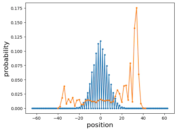
- This is a small example of the different behaviors of classical random walks and quantum walks.
Building a General Quantum Walk with Classiq
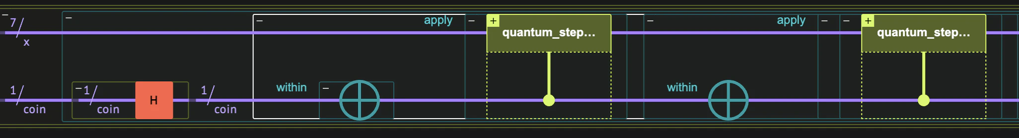
Define a quantum function for a discrete quantum walk. The arguments of the function:time: an integer for the number of walking steps.coin_flip_qfunc: the quantum function for “flipping” the coin.walks_qfuncs: a list of quantum functions for all possible transitions at a given point.coin_state: the quantum state of the coin.
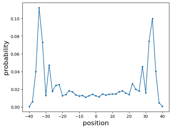
Example: Symmetric Quantum Walk on a Circle
As a first example, consider the circle geometry above, implemented with the generic definition but with a different initial condition for the coin. Take instead of . This state is a balanced initial condition for the coin (see Ref. [1]) and can be prepared by applying an H gate followed by an S gate.Output:
Output:
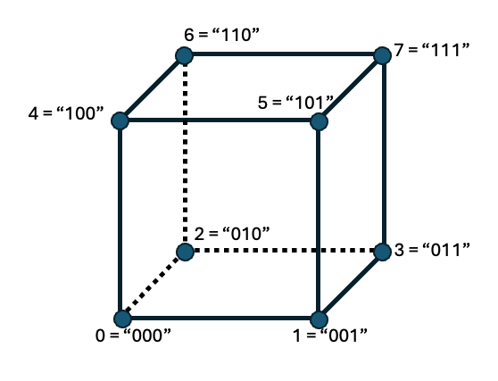
Example: 4D Hypercube with a Grover Coin
Next, consider a hypercube graph (see Figure 3). The quantum walk on a hypercube shows completely different behavior compared to its classical counterpart. One striking difference refers to the hitting time, which is the time it takes to reach node starting from an initial node . In particular, an interesting question is the hitting time between one corner of the hypercube “000..0” to the opposite one “111…1”. Ref. [2]) shows that the hitting time for the hypercube in quantum walks is exponentially faster than the analog quantity in classical random walks. The rigorous definition of the “hitting time” in the quantum case is nontrivial, and different definitions are relevant. This notebook does not use the exact definition, but simply demonstrates a specific result, highlighting the result of Ref. [2]. Define as the probability of measuring the walker at the opposite corner after steps, starting at position at time- Examine this quantity for the quantum and the classical case.
- Thus, a step along a hypercube is given by moving “1 Hamming distance away”.
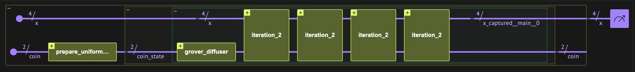
grover_diffuser function from the Classiq open library.
Output:
Output:
Output: