

View on GitHub
Open this notebook in GitHub to run it yourself
- Define a molecule and convert it into a Hamiltonian.
- Prepare the Hamiltonian for QPE, including normalization and trimming of negligible terms.
-
Construct a quantum model, initializing the state for the HF state and leveraging the
qpe_flexiblefunction. - Execute the circuit to find the related phases and analyze the results to find the ground state.
Defining a Molecule with Classiq
This tutorial works with the LiH molecule:Output:
Output:
Preparing the Molecule for QPE
Trimming the Hamiltonian
As you can see, the Hamiltonian may contain a large number of terms. In many cases you can compress the Hamiltonian by trimming small terms: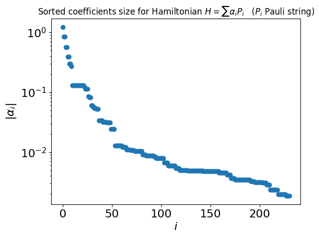
Output:
Normalizing the Hamiltonian for QPE
Since you are working with QPE, the ground state energy is inferred as a phase. Therefore, normalize the Hamiltonian so that its eigenvalues are in . This is done by finding a bound on the maximal absolute value of eigenvalues and normalizing the Hamiltonian by . A simple bound is given by the sum of Pauli coefficients of the Hamiltonian:Output:
Designing the Quantum Model
Defining a Powered Hamiltonian Simulation
Create a quantum model of the QPE algorithm using the Classiq platform, in particular, using the open library qpe_flexible function (and see this notebook as well). To approximate the Hamiltonian simulation , use the Classiq built-in implementation for Suzuki-Trotter formulas. For a given Suzuki-Trotter order , you can specify a repetition parameter that controls the level of approximation. The literature provides lower bounds for as a function of the operator error (defined by the diamond norm [3]). For example, Eq. (14) in Ref. [2] states that the Suzuki-Trotter formula of order 2 approximates up to an error , given repetitions that satisfies where . In particular, note that the number of repetitions grows as . In QPE, apply a powered Hamiltonian simulation: and approximate each power with Suzuki-Trotter for appropriate order and repetition parameters, keeping the same error per QPE iteration. You can thus use the bound above to define a powered Suzuki-Trotterqfunc for the specific molecule.
First, define a classical auxiliary function that help evaluate the right-hand-side side of Eq. (1):
Output:
Output:
Output:
Output:
Defining and Synthesizing the Phase Estimation Model
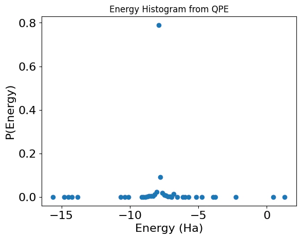
Measurement and Analysis
Execute on the default simulator:phase variable and multiplying back the normalization factor:
Output:
ASSUMED_OVERLAP*0.4 (0.4 is the case for ASSUMED_OVERLAP=1).
*Note that this is a very rough and simplistic analysis of the QPE algorithm result.
You can utilize more complex spectral analysis tools such as Gaussian mixtures.
Additional assumptions, such as the difference between adjacent eigenvalues or the number of overlapping eigenstates, can facilitate the analysis further.*
Output:
References
[1] [Michael A. Nielsen and Isaac L. Chuang. 2- Quantum Computation and Quantum Information: 10th Anniversary Edition, Cambridge University Press, New York, NY, USA. ](https://archive.org/details/QuantumComputationAndQuantumInformation10thAnniversaryEdition)