
View on GitHub

Open this notebook in GitHub to run it yourself
Integer Linear Programming (ILP) seeks a vector of integer numbers that maximizes (or minimizes) a linear cost function under a set of linear equality or inequality constraints [1]. In other words, it is an optimization problem where the cost function to optimize and all the constraints are linear and the decision variables are integers.

Mathematical Formulation

The ILP problem can be formulated as follows: given an nn-dimensional vector c=(c1,c2,,cn)\vec{c} = (c_1, c_2, \ldots, c_n), an m×nm \times n matrix A=(aij)A = (a_{ij}) with i=1,,mi=1,\ldots,m and j=1,,nj=1,\ldots,n, and an mm-dimensional vector b=(b1,b2,,bm)\vec{b} = (b_1, b_2, \ldots, b_m), find an nn-dimensional vector x=(x1,x2,,xn)\vec{x} = (x_1, x_2, \ldots, x_n) with integer entries that maximizes (or minimizes) the cost function: cx=c1x1+c2x2++cnxn\begin{align*} \vec{c} \cdot \vec{x} = c_1x_1 + c_2x_2 + \ldots + c_nx_n \end{align*} subject to these constraints: Axbxj0,j=1,2,,nxjZ,j=1,2,,n\begin{align*} A \vec{x} & \leq \vec{b} \\ x_j & \geq 0, \quad j = 1, 2, \ldots, n \\ x_j & \in \mathbb{Z}, \quad j = 1, 2, \ldots, n \end{align*} This tutorial guides you through the steps of solving the problem with the Classiq platform, using QAOA [2]. The solution is based on defining a Pyomo model for the optimization problem to solve.

Building the Pyomo Model from a Graph Input

Define the Pyomo model to use on the Classiq platform, using the mathematical formulation defined above:
import numpy as np
import pyomo.core as pyo


def ilp(a: np.ndarray, b: np.ndarray, c: np.ndarray, bound: int) -> pyo.ConcreteModel:
    # model constraint: a*x <= b
    model = pyo.ConcreteModel()
    assert b.ndim == c.ndim == 1

    num_vars = len(c)
    num_constraints = len(b)

    assert a.shape == (num_constraints, num_vars)

    model.x = pyo.Var(
        # here we bound x to be from 0 to to a given bound
        range(num_vars),
        domain=pyo.NonNegativeIntegers,
        bounds=(0, bound),
    )

    @model.Constraint(range(num_constraints))
    def monotone_rule(model, idx):
        return a[idx, :] @ list(model.x.values()) <= float(b[idx])

    # model objective: max(c * x)
    model.cost = pyo.Objective(expr=c @ list(model.x.values()), sense=pyo.maximize)

    return model

A = np.array([[1, 1, 1], [2, 2, 2], [3, 3, 3]])
b = np.array([1, 2, 3])
c = np.array([1, 2, 3])

# Instantiate the model
ilp_model = ilp(A, b, c, 3)

ilp_model.pprint()
Output:
1 Var Declarations
      x : Size=3, Index={0, 1, 2}
          Key : Lower : Value : Upper : Fixed : Stale : Domain
            0 :     0 :  None :     3 : False :  True : NonNegativeIntegers
            1 :     0 :  None :     3 : False :  True : NonNegativeIntegers
            2 :     0 :  None :     3 : False :  True : NonNegativeIntegers

  1 Objective Declarations
      cost : Size=1, Index=None, Active=True
          Key  : Active : Sense    : Expression
          None :   True : maximize : x[0] + 2*x[1] + 3*x[2]

  1 Constraint Declarations
      monotone_rule : Size=3, Index={0, 1, 2}, Active=True
          Key : Lower : Body                     : Upper : Active
            0 :  -Inf :       x[0] + x[1] + x[2] :   1.0 :   True
            1 :  -Inf : 2*x[0] + 2*x[1] + 2*x[2] :   2.0 :   True
            2 :  -Inf : 3*x[0] + 3*x[1] + 3*x[2] :   3.0 :   True

  3 Declarations: x monotone_rule cost
  

Setting Up the Classiq Problem Instance

To solve the Pyomo model defined above, use the CombinatorialProblem quantum object. Under the hood it translates the Pyomo model to a quantum model of QAOA, with the cost Hamiltonian translated from the Pyomo model. Choose the number of layers for the QAOA ansatz using the num_layers argument. The penalty_factor is the coefficient of the constraints term in the cost Hamiltonian.
from classiq import *
from classiq.applications.combinatorial_optimization import CombinatorialProblem

combi = CombinatorialProblem(pyo_model=ilp_model, num_layers=3, penalty_factor=10)

qmod = combi.get_model()

Synthesizing the QAOA Circuit and Solving the Problem

Synthesize and view the QAOA circuit (ansatz) used to solve the optimization problem:
qprog = combi.get_qprog()
show(qprog)
Output:

Quantum program link: https://platform.classiq.io/circuit/38w8GTGIHJELpFT0UWvNLftpCI6
  

Output:
https://platform.classiq.io/circuit/38w8GTGIHJELpFT0UWvNLftpCI6?login=True&version=15
  

Set the quantum backend on which to execute:
from classiq.execution import *

execution_preferences = ExecutionPreferences(
    backend_preferences=ClassiqBackendPreferences(backend_name="simulator"),
)
Solve the problem by calling the optimize method of the CombinatorialProblem object. For the classical optimization part of QAOA, define the maximum number of classical iterations (maxiter) and the α\alpha-parameter (quantile) for running CVaR-QAOA, an improved variation of QAOA [3]:
optimized_params = combi.optimize(execution_preferences, maxiter=90, quantile=0.7)
Check the convergence of the run:
import matplotlib.pyplot as plt

plt.plot(combi.cost_trace)
plt.xlabel("Iterations")
plt.ylabel("Cost")
plt.title("Cost convergence")
Output:

Text(0.5, 1.0, 'Cost convergence')
  

output

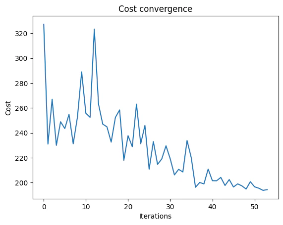
Optimization Results

Examine the statistics of the algorithm. The optimization is always defined as a minimization problem, so the positive maximization objective is translated to negative minimization by the Pyomo-to-Qmod translator. To get samples with the optimized parameters, call the sample method:
optimization_result = combi.sample(optimized_params)
optimization_result.sort_values(by="cost").head(5)
solutionprobabilitycost
12{‘x’: [0, 0, 1], ‘monotone_rule_1_slack_var’: …0.012207-3.0
223{‘x’: [0, 1, 0], ‘monotone_rule_1_slack_var’: …0.000488-2.0
146{‘x’: [1, 0, 0], ‘monotone_rule_1_slack_var’: …0.001953-1.0
15{‘x’: [0, 0, 0], ‘monotone_rule_1_slack_var’: …0.0117190.0
224{‘x’: [0, 0, 1], ‘monotone_rule_1_slack_var’: …0.0004887.0
Compare the optimized results to uniformly sampled results:
uniform_result = combi.sample_uniform()
And compare the histograms:
optimization_result["cost"].plot(
    kind="hist",
    bins=30,
    edgecolor="black",
    weights=optimization_result["probability"],
    alpha=0.6,
    label="optimized",
)
uniform_result["cost"].plot(
    kind="hist",
    bins=30,
    edgecolor="black",
    weights=uniform_result["probability"],
    alpha=0.6,
    label="uniform",
)
plt.legend()
plt.ylabel("Probability", fontsize=16)
plt.xlabel("cost", fontsize=16)
plt.tick_params(axis="both", labelsize=14)
output Plot the solution:
best_solution = optimization_result.solution[optimization_result.cost.idxmin()]
best_solution
Output:
{'x': [0, 0, 1],
   'monotone_rule_1_slack_var': [0],
   'monotone_rule_2_slack_var': [0]}
  

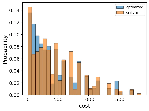
Comparing to a Classical Solver

Compare to the classical solution of the problem:
from pyomo.opt import SolverFactory

solver = SolverFactory("couenne")
solver.solve(ilp_model)
classical_solution = [int(pyo.value(ilp_model.x[i])) for i in range(len(ilp_model.x))]
print("Classical solution:", classical_solution)
Output:

Classical solution: [0, 0, 1]
  

References

[1] Integer Programming (Wikipedia). [2] Farhi, Edward, Jeffrey Goldstone, and Sam Gutmann. (2014). “A quantum approximate optimization algorithm.” arXiv preprint arXiv:1411.4028. [3] Barkoutsos, Panagiotis Kl, et al. (2020). “Improving variational quantum optimization using CVaR.” Quantum 4: 256.