
View on GitHub

Open this notebook in GitHub to run it yourself

Introduction

In the Number Partitioning Problem [1] we need to find how to partition a set of integers into two subsets of equal sums. In case such a partition does not exist, we can ask for a partition where the difference between the sums is minimal.

Mathematical formulation

Given a set of numbers S={s1,s2,...,sn}S=\{s_1,s_2,...,s_n\}, a partition is defined as P1,P2{1,...,n}P_1,P_2 \subset \{1,...,n\}, with P1P2={1,...,n}P_1\cup P_2=\{1,...,n\} and P1P2=P_1\cap P_2=\emptyset. In the Number Partitioning Problem we need to determine a partition such that jP1sjjP2sj|\sum_{j\in P_1}s_j-\sum_{j\in P_2}s_j| is minimal. A partition can be represented by a binary vector xx of size nn, where we assign 0 or 1 for being in P1P_1 or P2P_2, respectively. The quantity we ask to minimize is xs(1x)s=(2x1)s|\vec{x}\cdot \vec{s}-(1-\vec{x})\cdot\vec{s}|=|(2\vec{x}-1)\cdot\vec{s}|. In practice we will minimize the square of this expression.

Solving with the Classiq platform

We go through the steps of solving the problem with the Classiq platform, using QAOA algorithm [2]. The solution is based on defining a pyomo model for the optimization problem we would like to solve.
import networkx as nx
import numpy as np
import pyomo.core as pyo
from matplotlib import pyplot as plt

Building the Pyomo model from a graph input

We proceed by defining the Pyomo model that will be used on the Classiq platform, using the mathematical formulation defined above:
# we define a matrix which gets a set of integers s and returns a pyomo model for the partitioning problem


def partite(s) -> pyo.ConcreteModel:
    model = pyo.ConcreteModel()
    SetSize = len(s)  # the set size
    model.x = pyo.Var(
        range(SetSize), domain=pyo.Binary
    )  # our variable is a binary vector

    # we define a cost function
    model.cost = pyo.Objective(
        expr=sum(((2 * model.x[i] - 1) * s[i]) for i in range(SetSize)) ** 2,
        sense=pyo.minimize,
    )

    return model

Myset = np.random.randint(1, 12, 10)
mylist = [int(x) for x in Myset]
print("This is my list: ", mylist)
set_partition_model = partite(mylist)
Output:

This is my list:  [4, 5, 2, 10, 6, 11, 9, 4, 9, 1]
  

set_partition_model.pprint()
Output:
1 Var Declarations
      x : Size=10, Index={0, 1, 2, 3, 4, 5, 6, 7, 8, 9}
          Key : Lower : Value : Upper : Fixed : Stale : Domain
            0 :     0 :  None :     1 : False :  True : Binary
            1 :     0 :  None :     1 : False :  True : Binary
            2 :     0 :  None :     1 : False :  True : Binary
            3 :     0 :  None :     1 : False :  True : Binary
            4 :     0 :  None :     1 : False :  True : Binary
            5 :     0 :  None :     1 : False :  True : Binary
            6 :     0 :  None :     1 : False :  True : Binary
            7 :     0 :  None :     1 : False :  True : Binary
            8 :     0 :  None :     1 : False :  True : Binary
            9 :     0 :  None :     1 : False :  True : Binary

  1 Objective Declarations
      cost : Size=1, Index=None, Active=True
          Key  : Active : Sense    : Expression
          None :   True : minimize : ((2*x[0] - 1)*4 + (2*x[1] - 1)*5 + (2*x[2] - 1)*2 + (2*x[3] - 1)*10 + (2*x[4] - 1)*6 + (2*x[5] - 1)*11 + (2*x[6] - 1)*9 + (2*x[7] - 1)*4 + (2*x[8] - 1)*9 + (2*x[9] - 1))**2

  2 Declarations: x cost
  

Setting Up the Classiq Problem Instance

In order to solve the Pyomo model defined above, we use the CombinatorialProblem python class. Under the hood it tranlates the Pyomo model to a quantum model of the QAOA algorithm, with cost hamiltonian translated from the Pyomo model. We can choose the number of layers for the QAOA ansatz using the argument num_layers, and the penalty_factor, which will be the coefficient of the constraints term in the cost hamiltonian.
from classiq import *
from classiq.applications.combinatorial_optimization import CombinatorialProblem

combi = CombinatorialProblem(
    pyo_model=set_partition_model, num_layers=3, penalty_factor=10
)

qmod = combi.get_model()

Synthesizing the QAOA Circuit and Solving the Problem

We can now synthesize and view the QAOA circuit (ansatz) used to solve the optimization problem:
qprog = combi.get_qprog()
show(qprog)
Output:

Quantum program link: https://platform.classiq.io/circuit/38wAskQKdsHfkzDGJFSuT3lBDHt
  

Output:
https://platform.classiq.io/circuit/38wAskQKdsHfkzDGJFSuT3lBDHt?login=True&version=15
  

We also set the quantum backend we want to execute on:
from classiq.execution import *

execution_preferences = ExecutionPreferences(
    backend_preferences=ClassiqBackendPreferences(backend_name="simulator"),
)
We now solve the problem by calling the optimize method of the CombinatorialProblem object. For the classical optimization part of the QAOA algorithm we define the maximum number of classical iterations (maxiter) and the α\alpha-parameter (quantile) for running CVaR-QAOA, an improved variation of the QAOA algorithm [3]:
optimized_params = combi.optimize(execution_preferences, maxiter=80, quantile=0.7)
We can check the convergence of the run:
plt.plot(combi.cost_trace)
plt.xlabel("Iterations")
plt.ylabel("Cost")
plt.title("Cost convergence")
Output:

Text(0.5, 1.0, 'Cost convergence')
  

output

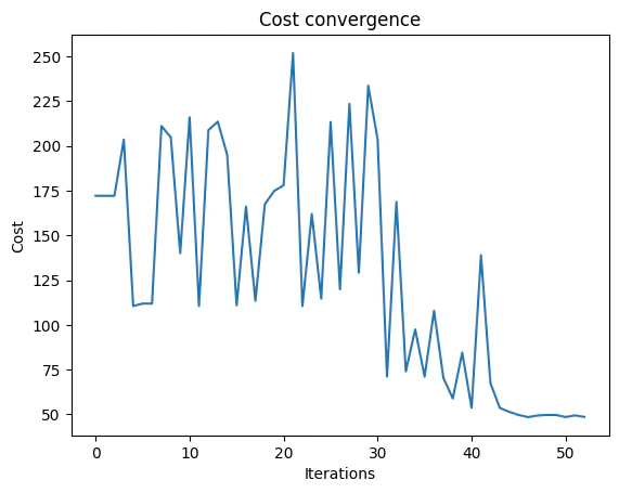
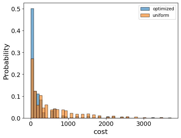
Optimization Results

We can also examine the statistics of the algorithm. In order to get samples with the optimized parameters, we call the sample method:
optimization_result = combi.sample(optimized_params)
optimization_result.sort_values(by="cost").head(5)
solutionprobabilitycost
0{‘x’: [1, 0, 0, 1, 0, 1, 0, 1, 0, 1]}0.0180661
88{‘x’: [1, 1, 0, 0, 0, 1, 1, 0, 0, 1]}0.0024411
263{‘x’: [0, 0, 1, 1, 1, 1, 0, 0, 0, 1]}0.0009771
285{‘x’: [1, 1, 1, 1, 1, 0, 0, 1, 0, 0]}0.0009771
287{‘x’: [0, 1, 0, 1, 1, 0, 1, 0, 0, 1]}0.0009771
We will also want to compare the optimized results to uniformly sampled results:
uniform_result = combi.sample_uniform()
And compare the histograms:
optimization_result["cost"].plot(
    kind="hist",
    bins=50,
    edgecolor="black",
    weights=optimization_result["probability"],
    alpha=0.6,
    label="optimized",
)
uniform_result["cost"].plot(
    kind="hist",
    bins=50,
    edgecolor="black",
    weights=uniform_result["probability"],
    alpha=0.6,
    label="uniform",
)
plt.legend()
plt.ylabel("Probability", fontsize=16)
plt.xlabel("cost", fontsize=16)
plt.tick_params(axis="both", labelsize=14)
output Let us plot the best solution:
best_solution = optimization_result.solution[optimization_result.cost.idxmin()]

p1 = [mylist[i] for i in range(len(mylist)) if best_solution["x"][i] == 0]
p2 = [mylist[i] for i in range(len(mylist)) if best_solution["x"][i] == 1]
print("P1=", p1, ", total sum: ", sum(p1))
print("P2=", p2, ", total sum: ", sum(p2))
print("difference= ", abs(sum(p1) - sum(p2)))
Output:

P1= [5, 2, 6, 9, 9] , total sum:  31
  P2= [4, 10, 11, 4, 1] , total sum:  30
  difference=  1
  

Lastly, we can compare to the classical solution of the problem:
from pyomo.opt import SolverFactory

solver = SolverFactory("couenne")
solver.solve(set_partition_model)

set_partition_model.display()
Output:

Model unknown

    Variables:
      x : Size=10, Index={0, 1, 2, 3, 4, 5, 6, 7, 8, 9}
          Key : Lower : Value : Upper : Fixed : Stale : Domain
            0 :     0 :   1.0 :     1 : False : False : Binary
            1 :     0 :   1.0 :     1 : False : False : Binary
            2 :     0 :   1.0 :     1 : False : False : Binary
            3 :     0 :   1.0 :     1 : False : False : Binary
            4 :     0 :   1.0 :     1 : False : False : Binary
            5 :     0 :   0.0 :     1 : False : False : Binary
            6 :     0 :   0.0 :     1 : False : False : Binary
            7 :     0 :   1.0 :     1 : False : False : Binary
            8 :     0 :   0.0 :     1 : False : False : Binary
            9 :     0 :   0.0 :     1 : False : False : Binary

    Objectives:
      cost : Size=1, Index=None, Active=True
          Key  : Active : Value
          None :   True :   1.0

    Constraints:
      None
  

classical_solution = [pyo.value(set_partition_model.x[i]) for i in range(len(mylist))]

p1 = [mylist[i] for i in range(len(mylist)) if round(classical_solution[i]) == 0]
p2 = [mylist[i] for i in range(len(mylist)) if round(classical_solution[i]) == 1]
print("P1=", p1, ", total sum: ", sum(p1))
print("P2=", p2, ", total sum: ", sum(p2))
print("difference= ", abs(sum(p1) - sum(p2)))
Output:

P1= [11, 9, 9, 1] , total sum:  30
  P2= [4, 5, 2, 10, 6, 4] , total sum:  31
  difference=  1
  

References

[1]: Number Partitioning Problem (Wikipedia) [2]: Farhi, Edward, Jeffrey Goldstone, and Sam Gutmann. “A quantum approximate optimization algorithm.” arXiv preprint arXiv:1411.4028 (2014). [3]: Barkoutsos, Panagiotis Kl, et al. “Improving variational quantum optimization using CVaR.” Quantum 4 (2020): 256.