

View on GitHub
Open this notebook in GitHub to run it yourself
Introduction and Background
In Finance models we are often interested in calculating the average of a function of a given probability distribution (). The most popular method to estimate the average is Monte Carlo [1] due to its flexibility and ability to generically handle stochastic parameters. Classical Monte Carlo methods, however, generally require extensive computational resources to provide an accurate estimation. By leveraging the laws of quantum mechanics, a quantum computer may provide novel ways to solve computationally intensive financial problems, such as risk management, portfolio optimization, and option pricing. The core quantum advantage of several of these applications is the Amplitude Estimation algorithm [2] which can estimate a parameter with a convergence rate of , compared to in the classical case, where is the number of Grover iterations in the quantum case and the number of the Monte Carlo samples in the classical case. This represents a theoretical quadratic speed-up of the quantum method over classical Monte Carlo methods!Option Pricing
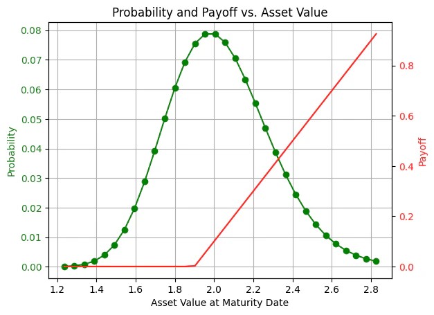
An option is the possibility to buy (call) or sell (put) an item (or share) at a known price - the strike price (K), where the option has a maturity price (S). The payoff function to describe for example a European call option will be: The maturity price is unknown. Therefore, it is expressed by a price distribution function, which may be any type of a distribution function. For example a log-normal distribution: , where is the standard normal distribution with mean equal to and standard deviation equal to .To estimate the average option price using a quantum computer, we need to:
- Load the distribution, that is, discretize the distribution using points (n is the number of qubits) and truncate it.
- Implement the payoff function that is equal to zero if and increases linearly otherwise.
- Evaluate the expected payoff using amplitude estimation.
Designing the Quantum Algorithm
In this workshop, we will collaboratively design a quantum algorithm to estimate the price of a European option. This algorithm can be applied to real-world stock data, providing practical results and offering a potential speedup over the classical Monte Carlo method. During the algorithm design process, you will explore state preparation and arithmetics, define Qstructs (quantum classes), and function calling using Classiq? The code in the following section is incomplete, with missing parts that you need to fill in, indicated by “#TODO” in the code description. If you’re unsure how to use a specific Classiq function, please refer to the Classiq documentation and search for the required quantum function to find its corresponding documentation page.The Probability Distribution
We begin by creating the probability distribution. The distribution is describing the option underlying asset price at maturity date. We will load a discrete version of the log-normal probability with points, when of the normal distribution is denoted bymu, by sigma and is the number of qubits num_qubits. K, the strike price, is also chosen in this section.
Output:
Output:
Quantum Function for Distribution Loading
Here we use the generalinplace_prepare_state function.
The inplace_prepare_state function is applied instead of prepare_state when a state preparation needs to be repeatedly applied to the same previously initialized quantum variable.
We use the genreal purpose state preparation for simplicity.
There are more efficient and scalable methods for preparing the required distribution, for example, see [4].
The Payoff Function
We now proceed to load the payoff function. Our end objective is to construct , which satisfies: Where is the quantum state of the maturity price (disregarding the prepared probability amplitudes for now) represented by a Qnum variable named ‘asset’ (see note), and the qubit state ( on the LHS) is represented by the ‘ind’ variable, serving as the indicator qubit. Due to the structure of the European option price payoff function, it is easily observed that the state remains unchanged if the maturity price is less than the strike price . For , on the other hand, a linear amplitude loading is applied to reflect the option’s payoff. *Note: in order to save qubits and depth, the register will hold a value in the range , effectively “labeling” the asset values. The mapping from the label space to the asset value space (and vice-versa) will occur within the comparator and amplitude loading, using the following (classical)scale/descale functions correspondingly*
assign_amplitude_table function.
While the calculation is accurate, it is not scalable for large variable sizes.
There are more scalable methods, like the ones mentioned in [4], [6].
*See Quantum Types in documentation (under Qmod reference) for Qstruct definition
Important: To ensure that the sum of all loaded amplitudes does not exceed 1, we normalize the payoff using a scaling_factor, which will later be multiplied during the post-processing stage.
Wrapping to an Amplitude Estimation model
After defining the probability distribution and the payoff function, we pack it into agrover_operator.
Both stages completed so far contribute to the state preparation process that precedes the successive applications of the Grover operator, an operator used to amplify the amplitudes of specific states corresponding to a desired output.
A Grover operator consists of two components: a phase oracle, which is used to distinguish between ‘good’ state and ‘bad’ states, and a diffusion operator, which reflects the states about the mean axis (usually achieved by some state preparation successively followed by a reflection about the state).
In our case, the oracle function is quite simple, and only needs to flip the sign when the indicator qubit is in the state (meaning )
After the initial probability and payoff loading, iterations of the Grover operator are applied within the Iterative Quantum Amplitude Estimation algorithm [5], which is a generalization of the Grover search algorithm, utilized for the estimation of the amplitude to arbitrary precision, given the state (now taking the prepared probability amplitudes into account):
Which approximates the expectation value of the payoff (after a post-processing step):
Quantum program synthesis
After we finished the model design, we synthesize the model to a quantum program.Output:
Quantum Program Execution
Finally, we execute with defined parameters for the accuracy of the amplitude estimation. This will affect the expected number of grover of repetitions within the execution, which is generally :Post processing
In order to get the expected payoff, we need to descale the measured amplitude byscaling_factor.
Output:
Compare to the expected calculated payoff
Output:
References
[1]: Paul Glasserman, Monte Carlo Methods in Financial Engineering. Springer-Verlag New York, 2003, p. 596.[2]: Gilles Brassard, Peter Hoyer, Michele Mosca, and Alain Tapp, Quantum Amplitude Amplification and Estimation. Contemporary Mathematics 305 (2002)
[3]: Nikitas Stamatopoulos, Daniel J. Egger, Yue Sun, Christa Zoufal, Raban Iten, Ning Shen, and Stefan Woerner, Option Pricing using Quantum Computers, Quantum 4, 291 (2020).
[4]: Chakrabarti, Shouvanik, et al. “A threshold for quantum advantage in derivative pricing.” Quantum 5 (2021): 463.
[5]: Grinko, D., Gacon, J., Zoufal, C. et al. Iterative quantum amplitude estimation. npj Quantum Inf 7, 52 (2021)
[6]: Francesca Cibrario et al., Quantum Amplitude Loading for Rainbow Options Pricing. Preprint