Min Graph Coloring Problem

View on GitHub

Open this notebook in GitHub to run it yourself

Background

Given a graph

G = (V,E)

, find the minimal number of colors k required to properly color it. A coloring is legal if:

each vetrex ${v_i}$ is assigned with a color $k_i \in \{0, 1, ..., k-1\}$
adajecnt vertex have different colors: for each $v_i, v_j$ such that $(v_i, v_j) \in E$ , $k_i \neq k_j$ . A graph which is k-colorable but not (k−1)-colorable is said to have chromatic number k.

The maximum bound on the chromatic number is

D_G + 1

, where

D_G

is the maximum vertex degree. The graph coloring problem is known to be in the NP-hard complexity class.

Solving the problem with classiq

Define the optimization problem

We encode the graph coloring with a matrix of variables X with dimensions

k \times |V|

using one-hot encoding, such that a

X_{ki} = 1

means that vertex i is colored by color k. We require that each vertex is colored by exactly one color and that 2 adjacent vertices have different colors.

import networkx as nx
import numpy as np
import pyomo.environ as pyo


def define_min_graph_coloring_model(graph, max_num_colors):
    model = pyo.ConcreteModel()

    nodes = list(graph.nodes())
    colors = range(0, max_num_colors)

    model.x = pyo.Var(colors, nodes, domain=pyo.Binary)
    x_variables = np.array(list(model.x.values()))

    adjacency_matrix = nx.convert_matrix.to_numpy_array(graph, nonedge=0)
    adjacency_matrix_block_diagonal = np.kron(np.eye(degree_max), adjacency_matrix)

    model.conflicting_color_constraint = pyo.Constraint(
        expr=x_variables @ adjacency_matrix_block_diagonal @ x_variables == 0
    )

    @model.Constraint(nodes)
    def each_vertex_is_colored(model, node):
        return sum(model.x[color, node] for color in colors) == 1

    def is_color_used(color):
        is_color_not_used = np.prod([(1 - model.x[color, node]) for node in nodes])
        return 1 - is_color_not_used

    # minimize the number of colors in use
    model.value = pyo.Objective(
        expr=sum(is_color_used(color) for color in colors), sense=pyo.minimize
    )

    return model

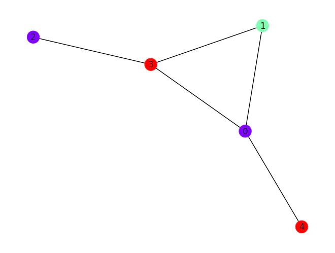
Initialize the model with example graph

graph = nx.erdos_renyi_graph(5, 0.3, seed=79)
nx.draw_kamada_kawai(graph, with_labels=True)

degree_sequence = sorted((d for n, d in graph.degree()), reverse=True)
degree_max = max(degree_sequence)
max_num_colors = degree_max

coloring_model = define_min_graph_coloring_model(graph, max_num_colors)

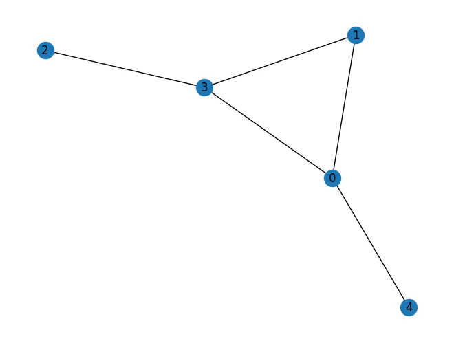
show the resulting pyomo model

coloring_model.pprint()

Output:

4 Set Declarations
      each_vertex_is_colored_index : Size=1, Index=None, Ordered=Insertion
          Key  : Dimen : Domain : Size : Members
          None :     1 :    Any :    5 : {0, 1, 2, 3, 4}
      x_index : Size=1, Index=None, Ordered=True
          Key  : Dimen : Domain              : Size : Members
          None :     2 : x_index_0*x_index_1 :   15 : {(0, 0), (0, 1), (0, 2), (0, 3), (0, 4), (1, 0), (1, 1), (1, 2), (1, 3), (1, 4), (2, 0), (2, 1), (2, 2), (2, 3), (2, 4)}
      x_index_0 : Size=1, Index=None, Ordered=Insertion
          Key  : Dimen : Domain : Size : Members
          None :     1 :    Any :    3 : {0, 1, 2}
      x_index_1 : Size=1, Index=None, Ordered=Insertion
          Key  : Dimen : Domain : Size : Members
          None :     1 :    Any :    5 : {0, 1, 2, 3, 4}

  1 Var Declarations
      x : Size=15, Index=x_index
          Key    : Lower : Value : Upper : Fixed : Stale : Domain
          (0, 0) :     0 :  None :     1 : False :  True : Binary
          (0, 1) :     0 :  None :     1 : False :  True : Binary
          (0, 2) :     0 :  None :     1 : False :  True : Binary
          (0, 3) :     0 :  None :     1 : False :  True : Binary
          (0, 4) :     0 :  None :     1 : False :  True : Binary
          (1, 0) :     0 :  None :     1 : False :  True : Binary
          (1, 1) :     0 :  None :     1 : False :  True : Binary
          (1, 2) :     0 :  None :     1 : False :  True : Binary
          (1, 3) :     0 :  None :     1 : False :  True : Binary
          (1, 4) :     0 :  None :     1 : False :  True : Binary
          (2, 0) :     0 :  None :     1 : False :  True : Binary
          (2, 1) :     0 :  None :     1 : False :  True : Binary
          (2, 2) :     0 :  None :     1 : False :  True : Binary
          (2, 3) :     0 :  None :     1 : False :  True : Binary
          (2, 4) :     0 :  None :     1 : False :  True : Binary

  1 Objective Declarations
      value : Size=1, Index=None, Active=True
          Key  : Active : Sense    : Expression
          None :   True : minimize : 1 - (1 - x[0,0])*(1 - x[0,1])*(1 - x[0,2])*(1 - x[0,3])*(1 - x[0,4]) + 1 - (1 - x[1,0])*(1 - x[1,1])*(1 - x[1,2])*(1 - x[1,3])*(1 - x[1,4]) + 1 - (1 - x[2,0])*(1 - x[2,1])*(1 - x[2,2])*(1 - x[2,3])*(1 - x[2,4])

  2 Constraint Declarations
      conflicting_color_constraint : Size=1, Index=None, Active=True
          Key  : Lower : Body                                                                                                                                                                                                                                                                                                                                                                                                   : Upper : Active
          None :   0.0 : (x[0,1] + x[0,3] + x[0,4])*x[0,0] + (x[0,0] + x[0,3])*x[0,1] + x[0,3]*x[0,2] + (x[0,0] + x[0,1] + x[0,2])*x[0,3] + x[0,0]*x[0,4] + (x[1,1] + x[1,3] + x[1,4])*x[1,0] + (x[1,0] + x[1,3])*x[1,1] + x[1,3]*x[1,2] + (x[1,0] + x[1,1] + x[1,2])*x[1,3] + x[1,0]*x[1,4] + (x[2,1] + x[2,3] + x[2,4])*x[2,0] + (x[2,0] + x[2,3])*x[2,1] + x[2,3]*x[2,2] + (x[2,0] + x[2,1] + x[2,2])*x[2,3] + x[2,0]*x[2,4] :   0.0 :   True
      each_vertex_is_colored : Size=5, Index=each_vertex_is_colored_index, Active=True
          Key : Lower : Body                     : Upper : Active
            0 :   1.0 : x[0,0] + x[1,0] + x[2,0] :   1.0 :   True
            1 :   1.0 : x[0,1] + x[1,1] + x[2,1] :   1.0 :   True
            2 :   1.0 : x[0,2] + x[1,2] + x[2,2] :   1.0 :   True
            3 :   1.0 : x[0,3] + x[1,3] + x[2,3] :   1.0 :   True
            4 :   1.0 : x[0,4] + x[1,4] + x[2,4] :   1.0 :   True

  8 Declarations: x_index_0 x_index_1 x_index x conflicting_color_constraint each_vertex_is_colored_index each_vertex_is_colored value
  

Setting Up the Classiq Problem Instance

In order to solve the Pyomo model defined above, we use the CombinatorialProblem python class. Under the hood it translates the Pyomo model to a quantum model of the QAOA algorithm [1], with cost hamiltonian translated from the Pyomo model. We can choose the number of layers for the QAOA ansatz using the argument num_layers.

from classiq import *
from classiq.applications.combinatorial_optimization import CombinatorialProblem

combi = CombinatorialProblem(pyo_model=coloring_model, num_layers=6, penalty_factor=10)

qmod = combi.get_model()

Synthesizing the QAOA Circuit and Solving the Problem

We can now synthesize and view the QAOA circuit (ansatz) used to solve the optimization problem:

qprog = combi.get_qprog()
show(qprog)

Output:

Quantum program link: https://platform.classiq.io/circuit/2zJB0wcTNTkUTnKwKPK0f4G7edG
  

We now solve the problem by calling the optimize method of the CombinatorialProblem object. For the classical optimization part of the QAOA algorithm we define the maximum number of classical iterations (maxiter) and the

\alpha

-parameter (quantile) for running CVaR-QAOA, an improved variation of the QAOA algorithm [2]:

optimized_params = combi.optimize(maxiter=100, quantile=0.7)

Output:


Optimization Progress: 101it [12:59,  7.72s/it]

We can check the convergence of the run:

import matplotlib.pyplot as plt

plt.plot(combi.cost_trace)
plt.xlabel("Iterations")
plt.ylabel("Cost")
plt.title("Cost convergence")

Output:


Text(0.5, 1.0, 'Cost convergence')

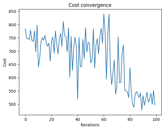
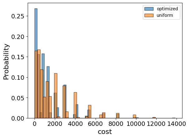
Optimization Results

We can also examine the statistics of the algorithm. In order to get samples with the optimized parameters, we call the sample method:

optimization_result = combi.sample(optimized_params)
optimization_result.sort_values(by="cost").head(5)

	solution	probability	cost
957	{‘x’: [[0, 1, 1, 0, 1], [1, 0, 0, 0, 0], [0, 0…	0.000488	3
1283	{‘x’: [[0, 1, 1, 0, 0], [0, 0, 0, 1, 1], [1, 0…	0.000488	3
1499	{‘x’: [[1, 0, 1, 0, 0], [0, 0, 0, 1, 0], [0, 1…	0.000488	3
376	{‘x’: [[1, 0, 1, 0, 0], [0, 1, 0, 0, 0], [0, 0…	0.000488	3
1435	{‘x’: [[1, 0, 1, 0, 0], [0, 0, 0, 1, 1], [0, 1…	0.000488	3

We will also want to compare the optimized results to uniformly sampled results:

uniform_result = combi.sample_uniform()

And compare the histograms:

optimization_result["cost"].plot(
    kind="hist",
    bins=50,
    edgecolor="black",
    weights=optimization_result["probability"],
    alpha=0.6,
    label="optimized",
)
uniform_result["cost"].plot(
    kind="hist",
    bins=50,
    edgecolor="black",
    weights=uniform_result["probability"],
    alpha=0.6,
    label="uniform",
)
plt.legend()
plt.ylabel("Probability", fontsize=16)
plt.xlabel("cost", fontsize=16)
plt.tick_params(axis="both", labelsize=14)

Let us plot the solution:

best_solution = optimization_result.solution[optimization_result.cost.idxmin()]
best_solution

Output:

{'x': [[1, 0, 1, 0, 0], [0, 1, 0, 0, 0], [0, 0, 0, 1, 1]]}

import matplotlib.pyplot as plt

best_solution = optimization_result.solution[optimization_result.cost.idxmin()]["x"]

one_hot_solution = np.array(best_solution).reshape([max_num_colors, len(graph.nodes)])
integer_solution = np.argmax(one_hot_solution, axis=0)
nx.draw_kamada_kawai(
    graph, with_labels=True, node_color=integer_solution, cmap=plt.cm.rainbow
)

References

[1]: Farhi, Edward, Jeffrey Goldstone, and Sam Gutmann. “A quantum approximate optimization algorithm.” arXiv preprint arXiv:1411.4028 (2014). [2]: Barkoutsos, Panagiotis Kl, et al. “Improving variational quantum optimization using CVaR.” Quantum 4 (2020): 256.

Algorithms

Applications

Functions

Tutorials

Min Graph Coloring Problem

View on GitHub

Background

Solving the problem with classiq

Define the optimization problem

Initialize the model with example graph

show the resulting pyomo model

Setting Up the Classiq Problem Instance

Synthesizing the QAOA Circuit and Solving the Problem

Optimization Results

References

Algorithms

Applications

Functions

Tutorials

View on GitHub

​Background

​Solving the problem with classiq

​

​Define the optimization problem

​

​Initialize the model with example graph

​

​show the resulting pyomo model

​Setting Up the Classiq Problem Instance

​Synthesizing the QAOA Circuit and Solving the Problem

​Optimization Results

​References

Background

Solving the problem with classiq

Define the optimization problem

Initialize the model with example graph

show the resulting pyomo model

Setting Up the Classiq Problem Instance

Synthesizing the QAOA Circuit and Solving the Problem

Optimization Results

References