

View on GitHub
Open this notebook in GitHub to run it yourself
Quantum Support Vector Machines is the quantum version of classical Support Vector Machines (SVM); i.e., a data classification method that separates the data by performing a mapping to a high-dimensional space, in which the data is separated by a hyperplane [1]. QSVM is a hybrid quantum–classical classification algorithm in which classical data are embedded into a high-dimensional quantum Hilbert space using a parameterized quantum feature map. A quantum processor is then used to evaluate inner products between these quantum states, producing a kernel matrix that captures similarities between data points in this quantum feature space. This kernel is passed to a classical support vector machine optimizer, which learns the optimal separating hyperplane by identifying support vectors and model parameters. For prediction, the trained model classifies new data points using quantum-evaluated kernel values and a classical decision rule. For some problem instances, a quantum feature map may enable improved classification performance while using fewer computational resources than a classical algorithm [2]. The algorithm treats the following problem:
- Input: Classical data points , where are d-dimensional vectors, corresponding labels , where , as well as feature map , encoding the classical data in a quantum state.
- Output: A kernel matrix evaluated using quantum measurements. The matrix is then fed into a classical SVM optimizer, producing a full characterization of the separating hyperplane.
Keywords: Quantum Machine Learning (QML), hybrid quantum–classical algorithm, supervised learning, binary classification.
Background
Our goal is to find a hyperplane in which separates the points into ones for which the corresponding labels are and . The hyperplane is conveniently defined by a vector normal to it, and an offset . The classification of a point can be determined by , which decides on which side of the hyperplane the point lies on. Here is the inner product between the two vectors. To describe the goal explicitly, we introduce the geometric margin as the distance from the hyperplane to the closest training point : . The optimal classification corresponds to the hyperplane and offset that maximizes the geometric margin. This goal can be stated as a naive optimization problem: find satisfying However, this formulation of the problem is a nonlinear optimization problem due to the sign comparison. Alternatively, we can express the objective as a linear function with linear constraints. A separating hyperplane satisfies moreover, we set the length of by enforcing that the inner product with respect to the nearest point (in fact, there will always be two data points on each side of the hyperplane with the same minimal distance to the hyperplane) to be . As a result, all data points satisfy . The condition enables defining the optimization problem In general, it would not be possible to separate the bare data points by a hyperplane; therefore, a transformation of the data to a higher-dimensional space using a feature map is performed. Following the transformation, the hyperplane and offset are evaluated (similar problem, obtained by transforming ). The main disadvantage of the present (primal) formulation of the problem is that explicitly computing may require infeasible computational resources, or even involve a mapping to an infinite-dimensional space. An alternative approach utilizes the dual formulation of the problem. This approach relies on the Karush-Kuhn-Tucker theorem [3], which implies that one can formulate a dual optimization problem, whose solution (under certain conditions which are satisfied for the present case) coincides with the solution of the present (primal) problem. The dual problem of the original primal optimization problem is given by where is the component of the matrix, called the kernel matrix. The important advantage of the dual formulation is that for specific feature maps, evaluation of the kernel matrix components does not require explicit assessment of the inner product of two feature vectors (which might be infinite-dimensional after the feature map transformation). The quantum version of SVM is based on the dual optimization problem, where the main innovation is that a quantum computer can perform unitary feature transformations by applying quantum circuits and evaluate the inner product between transformed states by specified measurements.QSVM Algorithms
The QSVM training algorithm includes three-steps.- Data loading of the classical data and feature map transformation.
- Evaluation of the overlap between two feature states.
- Classical optimization procedure, optimizing the circuit control parameters and modification of the feature map transformation.
QSVM with Classiq
We consider two kinds of 2D data sets:- A “simple” data set, constructed by randomly distributing points around two source data points.
- A more complex data set, generated by qiskit’s
ad_hoc_datafunction.
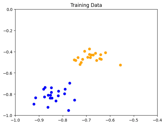
- In the first example, we generate “simple” artificial training, test, and prediction data sets (defined points in the data space). A Bloch sphere transformation is employed as a feature map, allowing perfect classification of the data.
- The second examples involve classifying the
ad_hoc_databy application of both the Bloch sphere and Pauli mappings.
Example 1: Bloch Sphere Feature Map Applied to Linearly Classifiable Data
We start coding with the relevant imports:- Training data: labelled data utilized to train and optimize the algorithm parameters
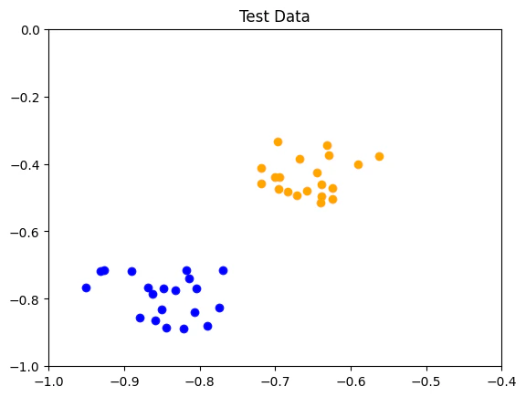
- Test data: labelled data employed to evaluate the optimization process
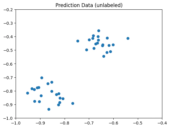
- Prediction data: unlabelled data that the optimized algorithm predicts the corresponding classification labels.
-
generate_data: given twosourcespoints and outputs a python dictionary with the training data points (random points within the vicinity of the sources). -
data_dict_to_data_and_labels: given a generated data dictionary, outputs the input data and associated labels.
Defining the Data
In addition to the feature map, we need to prepare our data. Thetraining_input and test_input datasets consist of data and its labels.
The labels are a 1D array where the value of the label corresponds to each data point and can be basically anything, such as (0, 1), (3, 5), or (‘A’, ‘B’).
The predict_input consists only of data points (without labels).
We normalize the data to be in the range .
Defining the Feature Map
When constructing a QSVM model, we must supply the feature map, encoding the classical data into quantum states in Hilbert space (the feature space of the problem). Here, we choose to encode the data onto the surface of the Bloch sphere. This can be defined in terms of the following transformation on the 2D data point where the circuit takes a single qubit per data point and the last equality is up to a global phase. We define a quantum function that generalizes the Bloch sphere mapping to an input vector of any dimension (also known as “dense angle encoding” in the field of quantum neural networks). Each pair of entries in the vector is mapped to a Bloch sphere. If there is an odd size, we apply a single RX gate on an extra qubit. Since a single qubit stores the data of a single data point, for such a feature mapping the number of qubits required is . The feature map is uploaded from theopen_library.functions.variational module at the beginning of the notebook.
Unlike the other feature maps, this feature map is located outside the quantum_feature_map module, as it serves as a building block beyond the scope of QSVM and QML.
Constructing a Model
We begin by building Classiq’sQSVM class, consisting of the QML model.
The model is given a feature map from the quantum_feature_maps module, and possibly ExecutionPreferences.
The feature map will be employed in the evaluation of the kernel in the training step.
Executing QSVM
The execution involves the following steps:- Training
- Testing the training process, and outputing a test score.
- Predicting, by taking unlabeled data and returning its predicted labels.
train, test and predict methods of the QSVM class.
In the training stage, the quantum kernel is constructed element by element, by repeated execution of quantum circuits.
The execution employs Classiq’s sample_batch to evaluate the overlap between the states encoding the two data points of each pair.
The kernel matrix is then fed into by scikit-learn’s SVC (Support Vector Classifier) function to optimize the quadratic program (the dual optimization problem).
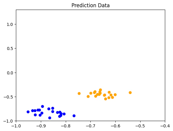
The knowledge of the optimized coefficients enables the model to predict the classification of a new data point, utilizing Eq. (1).
QSVM’s method get_qprog.
Output:
Results
We can view the classification accuracy throughtest_score, moreover, since this data was previously generated, we also know the real labels and can print them for comparison.
Output:
Example 2: Puali and Bloch Sphere Feature Map on a Complex Data Set
We begin by importing the relevant software packages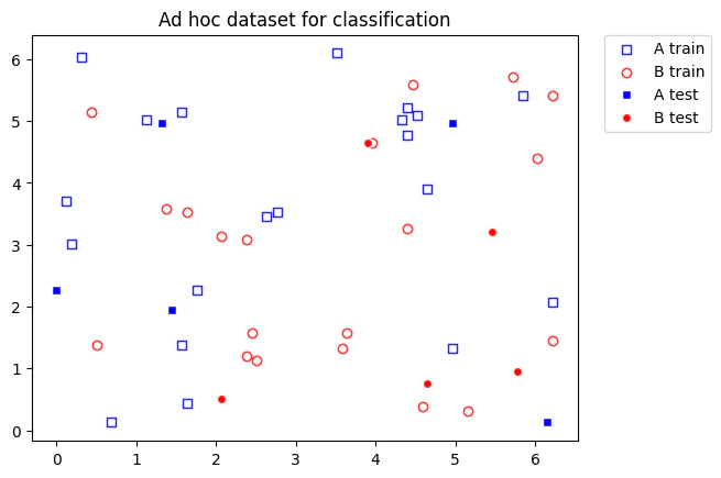
Pauli Feature Map
We build a Pauli feature map. This feature map is of size qubits for data of size , and it corresponds to the following unitary: where designates the Hadamard transform, and is a Hamiltonian acting on qubits according to some connectivity map, and is some classical function, typically taken as the polynomial of degree . For example, if our data is of size and we assume circular connectivity, taking Hamiltonians depending only on , the Hamiltonian reads as where and define some affine transformation on the data and correspond to the functions . We start by defining classical functions for creating a connectivity map for the Hamiltonians and for generating the full Hamiltonian:Model Construction
We firs define the hyperparameters of the Pauli feature map and construct an appropriate wrapper feature map, utilizingpauli_feature_map.
Train, Test and Prediction of the Pauli Model
Prediction Utilizing the Bloch Feature Map
We compare the Pauli feature map to the Bloch feature map results. For that end, we construct a new model, using theinplace_encode_on_bloch.
Results
The Pauli feature map accurately classifies the test and prediction data sets.Output:
Output:
Viewing the Model’s Parameterized Quantum Circuit
Output: