

View on GitHub
Open this notebook in GitHub to run it yourself
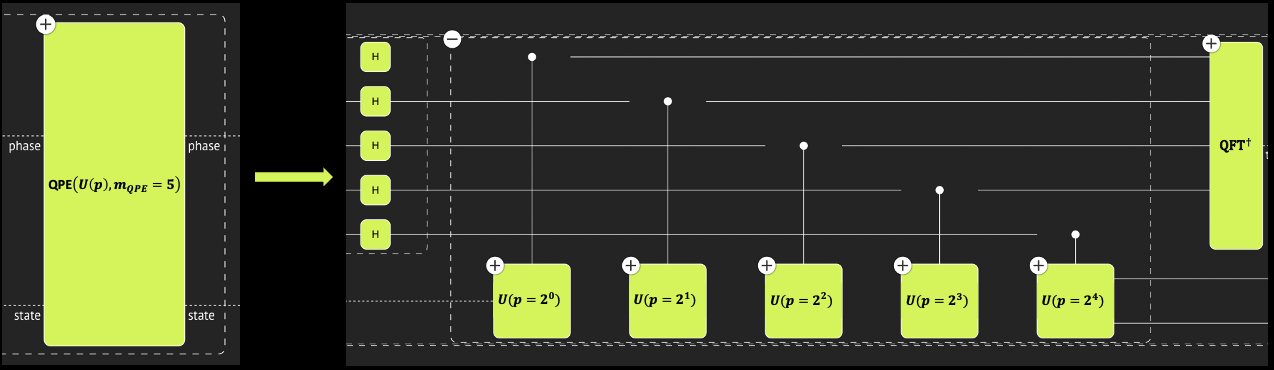
- Defining a Flexible QPE
- Example QPE for Finding the Eigenvalues of an Hermitian Matrix
2.1 Hamiltonian Evolution
Hamiltonian evolution, or Hamiltonian simulation, is one of the promising uses of quantum computers, where the advantage over classical approaches is clear and transparent (as proposed by Richard Feynman in 1982). Nevertheless, constructing a quantum program for efficient Hamiltonian dynamics is not an easy task. The most common examples use approximated product formulas such as the Trotter-Suzuki (TS) formulas.2.1.1 Trotter-Suzuki of Order 1
Write the Hamiltonian as a sum of Pauli strings , where are complex coefficients, and each of is a Pauli string of the form , with . Approximating Hamiltonian simulation with TS of order 1 refers to: where is called the number of repetitions.- Given a Hamiltonian and a functional error , what is the required number of repetitions?
- When performing a QPE, the challenge is even more pronounced:
2.1.2 A Flexible TS for Plugging into the Flexible QPE
The Trotter-Suzuki of order 1 function, , gets an Hamiltonian , evolution coefficient , and repetition . Define a wrapper function: The function tries to capture how many repetitions can approximate . Section 2.2 defines the “goodness of approximation”. Define ansatz for the repetition scaling : where , , and are parameters to tune.2.2 QPE Performance
In this tutorial, the measure for goodness of approximation refers to the functionality of the full QPE function, rather than taking a rigorous operator norm per each Hamiltonian simulation step in the QPE. Ways of examining the approximated QPE:- By its ability to approximate an eigenvalue for a given eigenvector.
- By comparing its resulting phase state with the one that results from a QPE with an exact Hamiltonian evolution, using a swap test.
- Exploring a Specific Example
PauliOperator object
Output:
*Note: For this example, the most naive upper bound for TS formula of order 1 and error (defined by a spectral norm) gives [2], with for the first QPE step. This corresponds to , and the following QPE steps grow exponentially . The result is a huge circuit depth, which you can relax by tuning the parameters of the ansatz.* Tighter bounds based on commutation relations[1] can give more reasonable numbers. However, the main purpose of this tutorial is to highlight the advantages of abstract, high-level modeling. Indeed, any known bound can be incorporated in the flexible Trotter-Suzuki by defining accordingly.
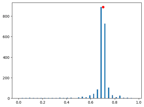
- Eigenvalue Estimation
Output:
Output:
- QPE State with Exact Hamiltonian Simulation Versus Approximated
Output:
Output:
- Comment
- This tutorial focused on the Trotter-Suzuki formula of order 1 for approximating the Hamiltonian simulation.