Max Colorable Induced Subgraph Problem

View on GitHub

Open this notebook in GitHub to run it yourself

Background

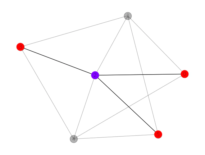
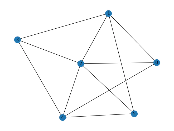
Given a graph

G = (V,E)

and number of colors K, find the largest induced subgraph that can be colored using up to K colors. A coloring is legal if:

each vetrex ${v_i}$ is assigned with a color $k_i \in \{0, 1, ..., k-1\}$
adajecnt vertex have different colors: for each $v_i, v_j$ such that $(v_i, v_j) \in E$ , $k_i \neq k_j$ .

An induced subgraph of a graph

G = (V,E)

is a graph

G'=(V', E')

such that

V'\subset V

and

E' = \{(v_1, v_2) \in E\ |\ v_1, v_2 \in V'\}

Define the optimization problem

import networkx as nx
import numpy as np
import pyomo.environ as pyo


def define_max_k_colorable_model(graph, K):
    model = pyo.ConcreteModel()

    nodes = list(graph.nodes())
    colors = range(0, K)

    # each x_i states if node i belongs to the cliques
    model.x = pyo.Var(colors, nodes, domain=pyo.Binary)
    x_variables = np.array(list(model.x.values()))

    adjacency_matrix = nx.convert_matrix.to_numpy_array(graph, nonedge=0)
    adjacency_matrix_block_diagonal = np.kron(np.eye(K), adjacency_matrix)

    # constraint that 2 nodes sharing an edge mustn't have the same color
    model.conflicting_color_constraint = pyo.Constraint(
        expr=x_variables @ adjacency_matrix_block_diagonal @ x_variables == 0
    )

    # each node should be colored
    @model.Constraint(nodes)
    def each_node_is_colored_once_or_zero(model, node):
        return sum(model.x[color, node] for color in colors) <= 1

    def is_node_colored(node):
        is_colored = np.prod([(1 - model.x[color, node]) for color in colors])
        return 1 - is_colored

    # maximize the number of nodes in the chosen clique
    model.value = pyo.Objective(
        expr=sum(is_node_colored(node) for node in nodes), sense=pyo.maximize
    )

    return model

Initialize the model with parameters

graph = nx.erdos_renyi_graph(6, 0.5, seed=7)
nx.draw_kamada_kawai(graph, with_labels=True)

NUM_COLORS = 2

coloring_model = define_max_k_colorable_model(graph, NUM_COLORS)

print the resulting pyomo model

coloring_model.pprint()

Output:

1 Var Declarations
      x : Size=12, Index={0, 1}*{0, 1, 2, 3, 4, 5}
          Key    : Lower : Value : Upper : Fixed : Stale : Domain
          (0, 0) :     0 :  None :     1 : False :  True : Binary
          (0, 1) :     0 :  None :     1 : False :  True : Binary
          (0, 2) :     0 :  None :     1 : False :  True : Binary
          (0, 3) :     0 :  None :     1 : False :  True : Binary
          (0, 4) :     0 :  None :     1 : False :  True : Binary
          (0, 5) :     0 :  None :     1 : False :  True : Binary
          (1, 0) :     0 :  None :     1 : False :  True : Binary
          (1, 1) :     0 :  None :     1 : False :  True : Binary
          (1, 2) :     0 :  None :     1 : False :  True : Binary
          (1, 3) :     0 :  None :     1 : False :  True : Binary
          (1, 4) :     0 :  None :     1 : False :  True : Binary
          (1, 5) :     0 :  None :     1 : False :  True : Binary

  1 Objective Declarations
      value : Size=1, Index=None, Active=True
          Key  : Active : Sense    : Expression
          None :   True : maximize : 1 - (1 - x[0,0])*(1 - x[1,0]) + 1 - (1 - x[0,1])*(1 - x[1,1]) + 1 - (1 - x[0,2])*(1 - x[1,2]) + 1 - (1 - x[0,3])*(1 - x[1,3]) + 1 - (1 - x[0,4])*(1 - x[1,4]) + 1 - (1 - x[0,5])*(1 - x[1,5])

  2 Constraint Declarations
      conflicting_color_constraint : Size=1, Index=None, Active=True
          Key  : Lower : Body                                                                                                                                                                                                                                                                                                                                                                                                                                                                                                                                                                                                                                                                                                                                                                                                                                                                                                                                                                                                                                                                                                                                                                                                                                                                                                                                                                                                                                                                                                                                                                                                                                                                                                                                                                                                                                                                      : Upper : Active
          None :   0.0 : (0.0*x[0,0] + x[0,1] + x[0,2] + 0.0*x[0,3] + x[0,4] + 0.0*x[0,5] + 0.0*x[1,0] + 0.0*x[1,1] + 0.0*x[1,2] + 0.0*x[1,3] + 0.0*x[1,4] + 0.0*x[1,5])*x[0,0] + (x[0,0] + 0.0*x[0,1] + x[0,2] + x[0,3] + 0.0*x[0,4] + x[0,5] + 0.0*x[1,0] + 0.0*x[1,1] + 0.0*x[1,2] + 0.0*x[1,3] + 0.0*x[1,4] + 0.0*x[1,5])*x[0,1] + (x[0,0] + x[0,1] + 0.0*x[0,2] + x[0,3] + x[0,4] + x[0,5] + 0.0*x[1,0] + 0.0*x[1,1] + 0.0*x[1,2] + 0.0*x[1,3] + 0.0*x[1,4] + 0.0*x[1,5])*x[0,2] + (0.0*x[0,0] + x[0,1] + x[0,2] + 0.0*x[0,3] + x[0,4] + 0.0*x[0,5] + 0.0*x[1,0] + 0.0*x[1,1] + 0.0*x[1,2] + 0.0*x[1,3] + 0.0*x[1,4] + 0.0*x[1,5])*x[0,3] + (x[0,0] + 0.0*x[0,1] + x[0,2] + x[0,3] + 0.0*x[0,4] + x[0,5] + 0.0*x[1,0] + 0.0*x[1,1] + 0.0*x[1,2] + 0.0*x[1,3] + 0.0*x[1,4] + 0.0*x[1,5])*x[0,4] + (0.0*x[0,0] + x[0,1] + x[0,2] + 0.0*x[0,3] + x[0,4] + 0.0*x[0,5] + 0.0*x[1,0] + 0.0*x[1,1] + 0.0*x[1,2] + 0.0*x[1,3] + 0.0*x[1,4] + 0.0*x[1,5])*x[0,5] + (0.0*x[0,0] + 0.0*x[0,1] + 0.0*x[0,2] + 0.0*x[0,3] + 0.0*x[0,4] + 0.0*x[0,5] + 0.0*x[1,0] + x[1,1] + x[1,2] + 0.0*x[1,3] + x[1,4] + 0.0*x[1,5])*x[1,0] + (0.0*x[0,0] + 0.0*x[0,1] + 0.0*x[0,2] + 0.0*x[0,3] + 0.0*x[0,4] + 0.0*x[0,5] + x[1,0] + 0.0*x[1,1] + x[1,2] + x[1,3] + 0.0*x[1,4] + x[1,5])*x[1,1] + (0.0*x[0,0] + 0.0*x[0,1] + 0.0*x[0,2] + 0.0*x[0,3] + 0.0*x[0,4] + 0.0*x[0,5] + x[1,0] + x[1,1] + 0.0*x[1,2] + x[1,3] + x[1,4] + x[1,5])*x[1,2] + (0.0*x[0,0] + 0.0*x[0,1] + 0.0*x[0,2] + 0.0*x[0,3] + 0.0*x[0,4] + 0.0*x[0,5] + 0.0*x[1,0] + x[1,1] + x[1,2] + 0.0*x[1,3] + x[1,4] + 0.0*x[1,5])*x[1,3] + (0.0*x[0,0] + 0.0*x[0,1] + 0.0*x[0,2] + 0.0*x[0,3] + 0.0*x[0,4] + 0.0*x[0,5] + x[1,0] + 0.0*x[1,1] + x[1,2] + x[1,3] + 0.0*x[1,4] + x[1,5])*x[1,4] + (0.0*x[0,0] + 0.0*x[0,1] + 0.0*x[0,2] + 0.0*x[0,3] + 0.0*x[0,4] + 0.0*x[0,5] + 0.0*x[1,0] + x[1,1] + x[1,2] + 0.0*x[1,3] + x[1,4] + 0.0*x[1,5])*x[1,5] :   0.0 :   True
      each_node_is_colored_once_or_zero : Size=6, Index={0, 1, 2, 3, 4, 5}, Active=True
          Key : Lower : Body            : Upper : Active
            0 :  -Inf : x[0,0] + x[1,0] :   1.0 :   True
            1 :  -Inf : x[0,1] + x[1,1] :   1.0 :   True
            2 :  -Inf : x[0,2] + x[1,2] :   1.0 :   True
            3 :  -Inf : x[0,3] + x[1,3] :   1.0 :   True
            4 :  -Inf : x[0,4] + x[1,4] :   1.0 :   True
            5 :  -Inf : x[0,5] + x[1,5] :   1.0 :   True

  4 Declarations: x conflicting_color_constraint each_node_is_colored_once_or_zero value
  

Setting Up the Classiq Problem Instance

In order to solve the Pyomo model defined above, we use the CombinatorialProblem python class. Under the hood it translates the Pyomo model to a quantum model of the QAOA algorithm [1], with cost hamiltonian translated from the Pyomo model. We can choose the number of layers for the QAOA ansatz using the argument num_layers.

from classiq import *
from classiq.applications.combinatorial_optimization import CombinatorialProblem

combi = CombinatorialProblem(pyo_model=coloring_model, num_layers=8)

qmod = combi.get_model()

Synthesizing the QAOA Circuit and Solving the Problem

We can now synthesize and view the QAOA circuit (ansatz) used to solve the optimization problem:

qprog = combi.get_qprog()
show(qprog)

Output:

Quantum program link: https://platform.classiq.io/circuit/38wA0LLtdYyT1s4HTKziIKBxF76
  

Output:

https://platform.classiq.io/circuit/38wA0LLtdYyT1s4HTKziIKBxF76?login=True&version=15
  

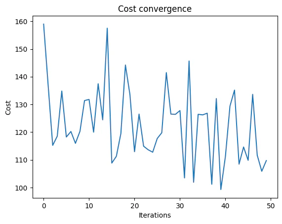
We now solve the problem by calling the optimize method of the CombinatorialProblem object. For the classical optimization part of the QAOA algorithm we define the maximum number of classical iterations (maxiter) and the

\alpha

-parameter (quantile) for running CVaR-QAOA, an improved variation of the QAOA algorithm [2]:

optimized_params = combi.optimize(maxiter=50, quantile=0.7)

We can check the convergence of the run:

import matplotlib.pyplot as plt

plt.plot(combi.cost_trace)
plt.xlabel("Iterations")
plt.ylabel("Cost")
plt.title("Cost convergence")

Output:


Text(0.5, 1.0, 'Cost convergence')

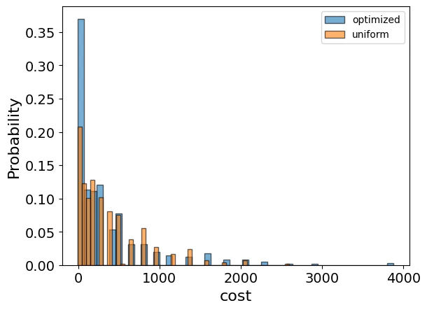
Optimization Results

We can also examine the statistics of the algorithm. The optimization is always defined as a minimzation problem, so the positive maximization objective was tranlated to a negative minimization one by the Pyomo to qmod translator. In order to get samples with the optimized parameters, we call the sample method:

optimization_result = combi.sample(optimized_params)
optimization_result.sort_values(by="cost").head(5)

	solution	probability	cost
109	{‘x’: [[0, 0, 1, 0, 0, 0], [1, 0, 0, 1, 0, 1]]}	0.001465	-4
237	{‘x’: [[0, 1, 0, 0, 1, 0], [1, 0, 0, 0, 0, 1]]}	0.000977	-4
1072	{‘x’: [[0, 1, 0, 0, 0, 0], [1, 0, 0, 1, 0, 1]]}	0.000488	-4
1118	{‘x’: [[1, 0, 0, 1, 0, 1], [0, 0, 1, 0, 0, 0]]}	0.000488	-4
386	{‘x’: [[0, 0, 0, 0, 1, 0], [1, 0, 0, 1, 0, 1]]}	0.000977	-4

We will also want to compare the optimized results to uniformly sampled results:

uniform_result = combi.sample_uniform()

And compare the histograms:

optimization_result["cost"].plot(
    kind="hist",
    bins=50,
    edgecolor="black",
    weights=optimization_result["probability"],
    alpha=0.6,
    label="optimized",
)
uniform_result["cost"].plot(
    kind="hist",
    bins=50,
    edgecolor="black",
    weights=uniform_result["probability"],
    alpha=0.6,
    label="uniform",
)
plt.legend()
plt.ylabel("Probability", fontsize=16)
plt.xlabel("cost", fontsize=16)
plt.tick_params(axis="both", labelsize=14)

Let us plot the best solution:

import matplotlib.pyplot as plt

best_solution = optimization_result.solution[optimization_result.cost.idxmin()]["x"]

one_hot_solution = np.array(best_solution).reshape([NUM_COLORS, len(graph.nodes)])
integer_solution = np.argmax(one_hot_solution, axis=0)

colored_nodes = np.array(graph.nodes)[one_hot_solution.sum(axis=0) != 0]
colors = integer_solution[colored_nodes]

pos = nx.kamada_kawai_layout(graph)
nx.draw(graph, pos=pos, with_labels=True, alpha=0.3, node_color="k")
nx.draw(graph.subgraph(colored_nodes), pos=pos, node_color=colors, cmap=plt.cm.rainbow)

References

[1]: Farhi, Edward, Jeffrey Goldstone, and Sam Gutmann. “A quantum approximate optimization algorithm.” arXiv preprint arXiv:1411.4028 (2014). [2]: Barkoutsos, Panagiotis Kl, et al. “Improving variational quantum optimization using CVaR.” Quantum 4 (2020): 256.

Algorithms

Applications

Functions

Tutorials

Max Colorable Induced Subgraph Problem

View on GitHub

Background

Define the optimization problem

Initialize the model with parameters

print the resulting pyomo model

Setting Up the Classiq Problem Instance

Synthesizing the QAOA Circuit and Solving the Problem

Optimization Results

References

Algorithms

Applications

Functions

Tutorials

View on GitHub

​Background

​Define the optimization problem

​

​Initialize the model with parameters

​

​print the resulting pyomo model

​Setting Up the Classiq Problem Instance

​Synthesizing the QAOA Circuit and Solving the Problem

​Optimization Results

​References

Background

Define the optimization problem

Initialize the model with parameters

print the resulting pyomo model

Setting Up the Classiq Problem Instance

Synthesizing the QAOA Circuit and Solving the Problem

Optimization Results

References