Max K-Vertex Cover

View on GitHub

Open this notebook in GitHub to run it yourself

Introduction

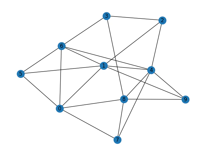
The Max K-Vertex Cover problem [1] is a classical problem in graph theory and computer science, where we aim to find a set of vertices such that each edge of the graph is incident to at least one vertex in the set, and the size of the set does not exceed a given number

k

Mathematical Formulation

The Max-k Vertex Cover problem can be formulated as an Integer Linear Program (ILP): Minimize:

\sum_{(i,j) \in E} (1 - x_i)(1 - x_j)

Subject to:

\sum_{i \in V} x_i = k

and

x_i \in \{0, 1\} \quad \forall i \in V

Where:

$x_i$ is a binary variable that equals 1 if node $i$ is in the cover and 0 otherwise
$E$ is the set of edges in the graph
$V$ is the set of vertices in the graph
$k$ is the maximum number of vertices allowed in the cover

Solving with the Classiq platform

We go through the steps of solving the problem with the Classiq platform, using QAOA algorithm [2]. The solution is based on defining a Pyomo model for the optimization problem we would like to solve.

import networkx as nx
import numpy as np
import pyomo.core as pyo
from IPython.display import Markdown, display
from matplotlib import pyplot as plt

Building the Pyomo model from a graph input

We proceed by defining the Pyomo model that will be used on the Classiq platform, using the mathematical formulation defined above:

def mvc(graph: nx.Graph, k: int) -> pyo.ConcreteModel:
    model = pyo.ConcreteModel()
    model.x = pyo.Var(graph.nodes, domain=pyo.Binary)
    model.amount_constraint = pyo.Constraint(expr=sum(model.x.values()) == k)

    def obj_expression(model):
        # number of edges not covered
        return sum((1 - model.x[i]) * (1 - model.x[j]) for i, j in graph.edges)

    model.cost = pyo.Objective(rule=obj_expression, sense=pyo.minimize)

    return model

The model contains:

Index set declarations (model.Nodes, model.Arcs).
Binary variable declaration for each node (model.x) indicating whether the variable is chosen for the set.
Constraint rule – ensures that the set is of size k.
Objective rule – counts the number of edges not covered; i.e., both related variables are zero.

K = 5
num_nodes = 10
p_edge = 0.5
graph = nx.erdos_renyi_graph(n=num_nodes, p=p_edge, seed=13)

nx.draw_kamada_kawai(graph, with_labels=True)
mvc_model = mvc(graph, K)

mvc_model.pprint()

Output:

1 Var Declarations
      x : Size=10, Index={0, 1, 2, 3, 4, 5, 6, 7, 8, 9}
          Key : Lower : Value : Upper : Fixed : Stale : Domain
            0 :     0 :  None :     1 : False :  True : Binary
            1 :     0 :  None :     1 : False :  True : Binary
            2 :     0 :  None :     1 : False :  True : Binary
            3 :     0 :  None :     1 : False :  True : Binary
            4 :     0 :  None :     1 : False :  True : Binary
            5 :     0 :  None :     1 : False :  True : Binary
            6 :     0 :  None :     1 : False :  True : Binary
            7 :     0 :  None :     1 : False :  True : Binary
            8 :     0 :  None :     1 : False :  True : Binary
            9 :     0 :  None :     1 : False :  True : Binary

  1 Objective Declarations
      cost : Size=1, Index=None, Active=True
          Key  : Active : Sense    : Expression
          None :   True : minimize : (1 - x[0])*(1 - x[1]) + (1 - x[0])*(1 - x[5]) + (1 - x[0])*(1 - x[6]) + (1 - x[0])*(1 - x[7]) + (1 - x[0])*(1 - x[8]) + (1 - x[1])*(1 - x[2]) + (1 - x[1])*(1 - x[4]) + (1 - x[1])*(1 - x[5]) + (1 - x[1])*(1 - x[6]) + (1 - x[1])*(1 - x[9]) + (1 - x[2])*(1 - x[3]) + (1 - x[2])*(1 - x[4]) + (1 - x[3])*(1 - x[6]) + (1 - x[3])*(1 - x[8]) + (1 - x[4])*(1 - x[6]) + (1 - x[4])*(1 - x[7]) + (1 - x[4])*(1 - x[8]) + (1 - x[4])*(1 - x[9]) + (1 - x[5])*(1 - x[6]) + (1 - x[7])*(1 - x[8]) + (1 - x[8])*(1 - x[9])

  1 Constraint Declarations
      amount_constraint : Size=1, Index=None, Active=True
          Key  : Lower : Body                                                                : Upper : Active
          None :   5.0 : x[0] + x[1] + x[2] + x[3] + x[4] + x[5] + x[6] + x[7] + x[8] + x[9] :   5.0 :   True

  3 Declarations: x amount_constraint cost
  

Setting Up the Classiq Problem Instance

In order to solve the Pyomo model defined above, we use the CombinatorialProblem python class. Under the hood it tranlates the Pyomo model to a quantum model of the QAOA algorithm, with cost hamiltonian translated from the Pyomo model. We can choose the number of layers for the QAOA ansatz using the argument num_layers, and the penalty_factor, which will be the coefficient of the constraints term in the cost hamiltonian.

from classiq import *
from classiq.applications.combinatorial_optimization import CombinatorialProblem

combi = CombinatorialProblem(pyo_model=mvc_model, num_layers=3, penalty_factor=10)

qmod = combi.get_model()

Synthesizing the QAOA Circuit and Solving the Problem

We can now synthesize and view the QAOA circuit (ansatz) used to solve the optimization problem:

qprog = combi.get_qprog()
show(qprog)

Output:

Quantum program link: https://platform.classiq.io/circuit/38wAZjti7TSIt7NXGCJaFgelCqw
  

Output:

https://platform.classiq.io/circuit/38wAZjti7TSIt7NXGCJaFgelCqw?login=True&version=15
  

We also set the quantum backend we want to execute on:

from classiq.execution import *

execution_preferences = ExecutionPreferences(
    backend_preferences=ClassiqBackendPreferences(backend_name="simulator"),
)

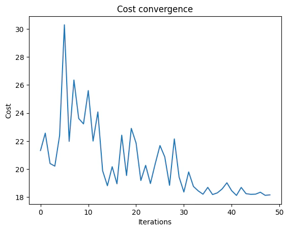
We now solve the problem by calling the optimize method of the CombinatorialProblem object. For the classical optimization part of the QAOA algorithm we define the maximum number of classical iterations (maxiter) and the

\alpha

-parameter (quantile) for running CVaR-QAOA, an improved variation of the QAOA algorithm [3]:

optimized_params = combi.optimize(execution_preferences, maxiter=90, quantile=0.7)

We can check the convergence of the run:

import matplotlib.pyplot as plt

plt.plot(combi.cost_trace)
plt.xlabel("Iterations")
plt.ylabel("Cost")
plt.title("Cost convergence")

Output:


Text(0.5, 1.0, 'Cost convergence')

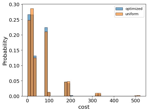
Optimization Results

We can also examine the statistics of the algorithm. In order to get samples with the optimized parameters, we call the sample method:

optimization_result = combi.sample(optimized_params)
optimization_result.sort_values(by="cost").head(5)

	solution	probability	cost
194	{‘x’: [1, 1, 0, 1, 1, 0, 0, 0, 1, 0]}	0.001953	1
191	{‘x’: [1, 1, 0, 1, 1, 0, 1, 0, 0, 0]}	0.001953	2
465	{‘x’: [0, 1, 0, 0, 1, 0, 1, 1, 1, 0]}	0.000488	2
444	{‘x’: [0, 1, 0, 1, 1, 1, 0, 0, 1, 0]}	0.000977	2
609	{‘x’: [1, 1, 1, 0, 1, 0, 0, 0, 1, 0]}	0.000488	2

We will also want to compare the optimized results to uniformly sampled results:

uniform_result = combi.sample_uniform()

And compare the histograms:

optimization_result["cost"].plot(
    kind="hist",
    bins=40,
    edgecolor="black",
    weights=optimization_result["probability"],
    alpha=0.6,
    label="optimized",
)
uniform_result["cost"].plot(
    kind="hist",
    bins=40,
    edgecolor="black",
    weights=uniform_result["probability"],
    alpha=0.6,
    label="uniform",
)
plt.legend()
plt.ylabel("Probability", fontsize=16)
plt.xlabel("cost", fontsize=16)
plt.tick_params(axis="both", labelsize=14)

Let us plot the solution:

best_solution = optimization_result.solution[optimization_result.cost.idxmin()]["x"]
best_solution

Output:

[1, 1, 0, 1, 1, 0, 0, 0, 1, 0]

def draw_solution(graph: nx.Graph, solution: list):
    solution_nodes = [v for v in graph.nodes if solution[v]]
    solution_edges = [
        (u, v) for u, v in graph.edges if u in solution_nodes or v in solution_nodes
    ]
    nx.draw_kamada_kawai(graph, with_labels=True)
    nx.draw_kamada_kawai(
        graph,
        nodelist=solution_nodes,
        edgelist=solution_edges,
        node_color="r",
        edge_color="y",
    )


draw_solution(graph, best_solution)

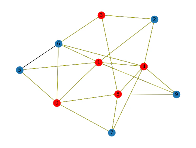
Comparison to a classical solver

Lastly, we can compare to the classical solution of the problem:

from pyomo.opt import SolverFactory

solver = SolverFactory("couenne")
solver.solve(mvc_model)
classical_solution = [int(pyo.value(mvc_model.x[i])) for i in graph.nodes]


classical_solution

Output:

[1, 1, 0, 1, 1, 0, 0, 0, 1, 0]

draw_solution(graph, classical_solution)

References

[1]: Max k-Vertex Cover. [2]: Farhi, Edward, Jeffrey Goldstone, and Sam Gutmann. “A quantum approximate optimization algorithm.” arXiv preprint arXiv:1411.4028 (2014). [3]: Barkoutsos, Panagiotis Kl, et al. “Improving variational quantum optimization using CVaR.” Quantum 4 (2020): 256.

Algorithms

Applications

Functions

Tutorials

View on GitHub

Introduction

Mathematical Formulation

Solving with the Classiq platform

Building the Pyomo model from a graph input

Setting Up the Classiq Problem Instance

Synthesizing the QAOA Circuit and Solving the Problem

Optimization Results

Comparison to a classical solver

References

Algorithms

Applications

Functions

Tutorials

View on GitHub

​Introduction

​

​Mathematical Formulation

​Solving with the Classiq platform

​Building the Pyomo model from a graph input

​Setting Up the Classiq Problem Instance

​Synthesizing the QAOA Circuit and Solving the Problem

​Optimization Results

​Comparison to a classical solver

​References

Introduction

Mathematical Formulation

Solving with the Classiq platform

Building the Pyomo model from a graph input

Setting Up the Classiq Problem Instance

Synthesizing the QAOA Circuit and Solving the Problem

Optimization Results

Comparison to a classical solver

References