

View on GitHub
Open this notebook in GitHub to run it yourself
This tutorial delves into a technique for tackling the challenge of solving WSN link monitoring through the lens of the Minimum Vertex Cover (MVC) problem using Classiq.
The Link Monitoring Problem
WSNs do not have a predefined structure to maintain fundamental data-transfer operations. They are crucial communication layer technologies for providing environmental sensing operations in the IoT. Most of the time, WSNs are deployed for various applications in forests, mines, and land borders, where they must bear harsh circumstances. Link monitoring in WSNs involves identifying the optimal set of communication links between sensors to guarantee reliable data transmission while minimizing energy use. As the network scales, manually selecting these links becomes increasingly complex and time-consuming. This is where the concept of graph theory and the MVC problem step in.Graph Modeling
To effectively address the link monitoring challenge, this tutorial leverages graph theory to model the WSN. Each sensor is represented as a node, and communication links between sensors are depicted as edges. This graphical representation captures the essence of connectivity in the network, providing a foundation for optimizing link monitoring. A WSN can be modeled as a graph , where and represent the set of vertices (nodes) and edges (communication links), respectively. A vertex cover of a given undirected graph is a set where each is incident to at least one vertex of .MVC Concept
At the heart of the approach lies the concept of the Minimum Vertex Cover [2]. This optimization problem aims to find the smallest subset of nodes (vertices) in a graph such that every edge in the graph is incident to at least one of these nodes. In the context of WSNs, the vertices selected for the MVC represent the critical sensors that ensure seamless communication throughout the network.Vertex cover is a useful structure for WSN applications such as routing, clustering, backbone formation, link monitoring, replica management, and network attack protection.
Working Example
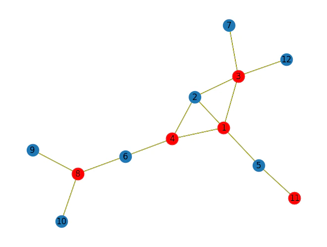
An example of sensor network deployment for a habitat monitoring application is depicted in Figure 1(a), where there are nodes in the sensing area and node is the sink node. The graph representation of this network is given in Figure 1(b). Figure 1(c) shows the link monitoring application for this topology. In this application, each link must be sniffed by one secure point (monitor node) to detect attacks such as packet injection and data manipulation. The red nodes (nodes , and ) are secure points assigned to control message traffic in Figure 1(c). Red arrows show the assigned links to the monitor nodes in the same figure. For example, the links and are monitored by node . This architecture can also be used in other common operations such as backbone formation, clustering, and routing. Red nodes can be cluster heads, and ordinary nodes can send their data to the cluster heads to achieve data aggregation. The network induced by red nodes is a virtual backbone that can carry messages to the sink node. By accomplishing the clustering and backbone formation operations, the data packets can be routed from ordinary nodes to the sink node.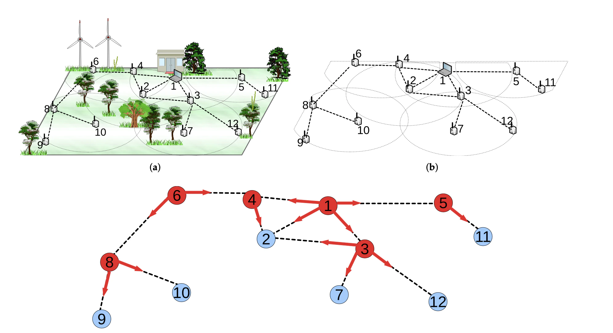
Figure
- An example of a link monitoring application for the vertex cover problem: (a) Deployment of a sample WSN; (b) Graph representation of the topology; (c) Link monitoring application on the topology.
MVC Mathematical Formulation
The MVC problem can be formulated as a Quadratic Unconstrained Binary Optimization (QUBO): Minimize: Subject to: and Where:- is a binary variable that equals 1 if node is in the cover and 0 otherwise
- is the set of all edges (connected and not connected)
- is the set of vertices in the graph
Solving MVC with Classiq and QAOA
Follow the steps for solving the MVC problem with Classiq using the Quantum Approximate Optimization Algorithm (QAOA) [2]. QAOA is a quantum algorithm designed to solve combinatorial optimization problems, making it an ideal candidate for tackling the MVC problem in large-scale WSNs. Apply QAOA to the modeled graph, iteratively adjusting the parameters to navigate the solution space and identify the MVC. Quantum computing’s unique ability to explore multiple solution candidates simultaneously accelerates the optimization process, significantly outperforming classical algorithms for complex problems. To solve the link monitoring problem with Classiq:- Build a Classiq model.
- Generate a parameterized quantum circuit.
- Execute the circuit and optimize parameters to get the optimal solution.
Building the Working Example Graph
Build and view a modeled graph to fit the working example above: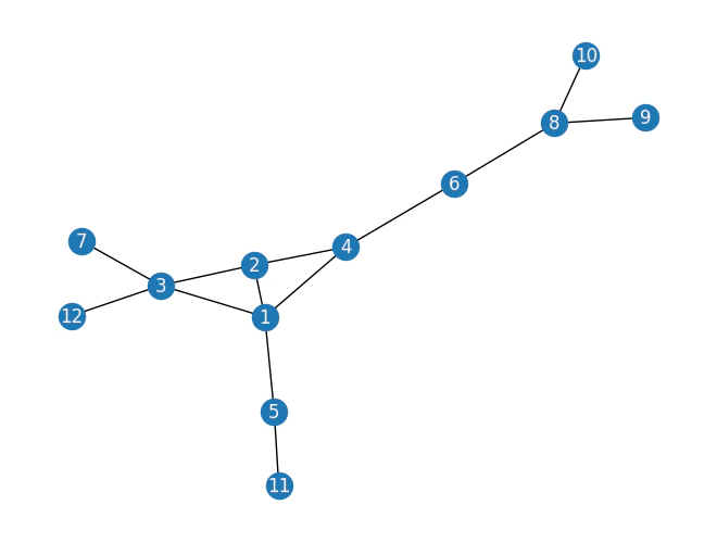
Building the Optimization Model from Graph Input
To build the optimization model, use Pyomo, a Python-based, open-source optimization modeling language with a diverse set of optimization capabilities. Formalize the QUBO model into a Pyomo model object. Classiq seamlessly incorporates the Pyomo object into its model. Define the Pyomo model that is used to build a Classiq model using the mathematical formulation defined above:- a binary variable declaration for each node (model.x), indicating whether the variable is chosen for the set.
- a constraint rule ensuring that all edges are covered.
- an objective rule that minimizes the number of selected nodes.
Output:
- Building a Classiq Model
construct_combinatorial_optimization_model function to create the model object.
As input for this function, define the quantum configuration of the QAOA algorithm though the QAOAConfig object where the number of repetitions (num_layers) is defined:
OptimizerConfig object where the maximum number of classical iterations (max_iteration) and the -parameter (alpha_cvar) for running CVaR-QAOA—an improved variation of the QAOA algorithm [3]—are defined:
qmod) already incorporates the QAOA execution logic. However, you can set the quantum backend on which to execute so the Classiq synthesis engine takes it into consideration when generating an optimized quantum circuit:
That’s it! The Classiq model is set!!
- Generating a Parameterized Quantum Circuit
synthesize the model and view the QAOA circuit (ansatz) used to solve the optimization problem:
Output:
- Executing the Circuit: Optimizing Parameters to Get the Optimal Solution
execute method:
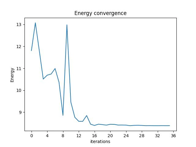
- Analyzing the Energy Convergence Execution Results
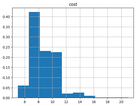
| probability | cost | solution | count | |
|---|---|---|---|---|
| 37 | 0.002930 | 5.0 | [1, 0, 1, 1, 1, 0, 0, 1, 0, 0, 0, 0] | 6 |
| 2 | 0.004395 | 5.0 | [1, 0, 1, 1, 0, 0, 0, 1, 0, 0, 1, 0] | 9 |
| 10 | 0.003906 | 5.0 | [0, 1, 1, 1, 1, 0, 0, 1, 0, 0, 0, 0] | 8 |
| 104 | 0.002441 | 6.0 | [1, 0, 1, 1, 1, 0, 0, 1, 0, 0, 0, 1] | 5 |
| 96 | 0.002441 | 6.0 | [1, 0, 1, 1, 1, 0, 0, 1, 0, 1, 0, 0] | 5 |
Output:
Output:
Output:
You obtained a set of vertices that form the MVC! These vertices correspond to the critical sensors that need to be monitored and maintained for optimal link connectivity.The outcome is a comprehensive link monitoring strategy that ensures efficient data transmission while conserving energy.