Hello Many Worlds
With Classiq (as, perhaps, with quantum computing) there are many parallel worlds in which to work; specifically, the IDE and Python SDK interfaces. The 'Hello World' example below runs in different flows of the design-optimize-analyze-execute steps between the IDE and the Python SDK:
-
Design (SDK) - Optimize (SDK) - Analyze (IDE) - Execute (SDK)
-
Design (SDK) - Optimize (SDK) - Analyze (IDE) - Execute (IDE)
The 'Hello World' example calculates the simple arithmetic operation \(y=x^2+1\) in a superposition. This example is covered in depth in Classiq 101.
All in IDE
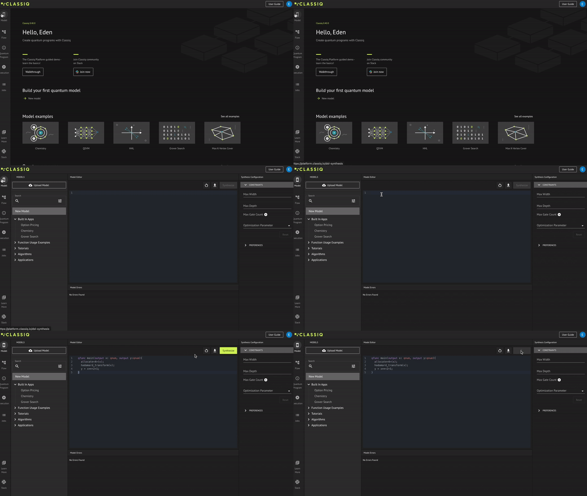
Copy and paste the following code in the Model tab in the IDE, then click Synthesize as shown in the GIF:
qfunc main(output x: qnum, output y:qnum){
  allocate(4, x);
  hadamard_transform(x);
  y = x**2+1;
}
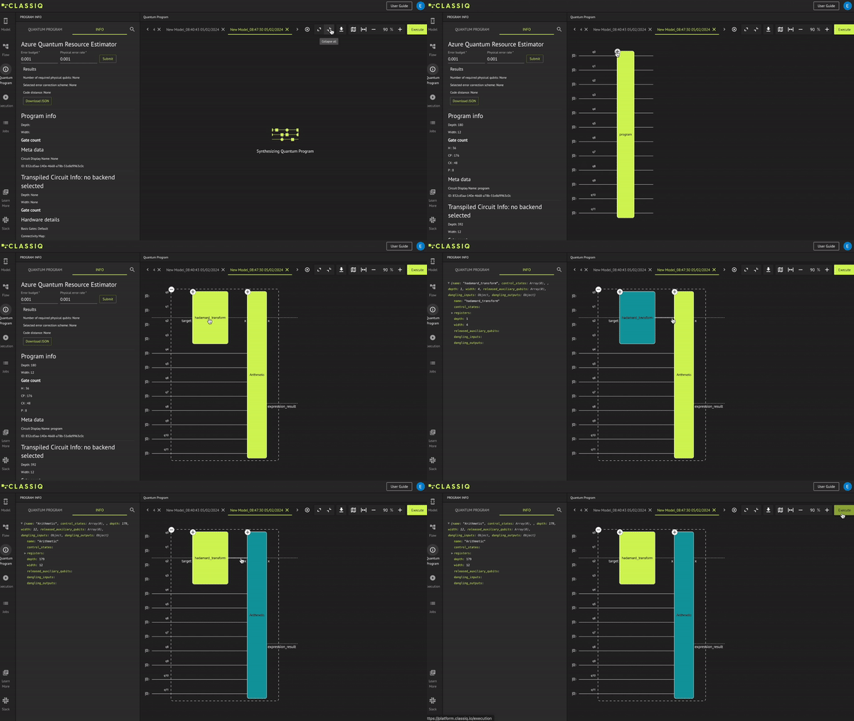
Check that you receive two blocks in the quantum circuit: hadamard_transform and Arithmetic, then click Execute:
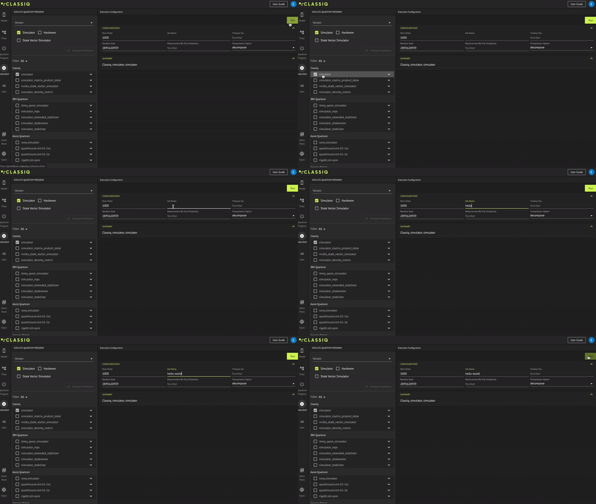
In the Execution tab, under the Classiq provider, choose the simulator (and make sure that other options are not selected). Change the job name to 'hello world' and click Run:
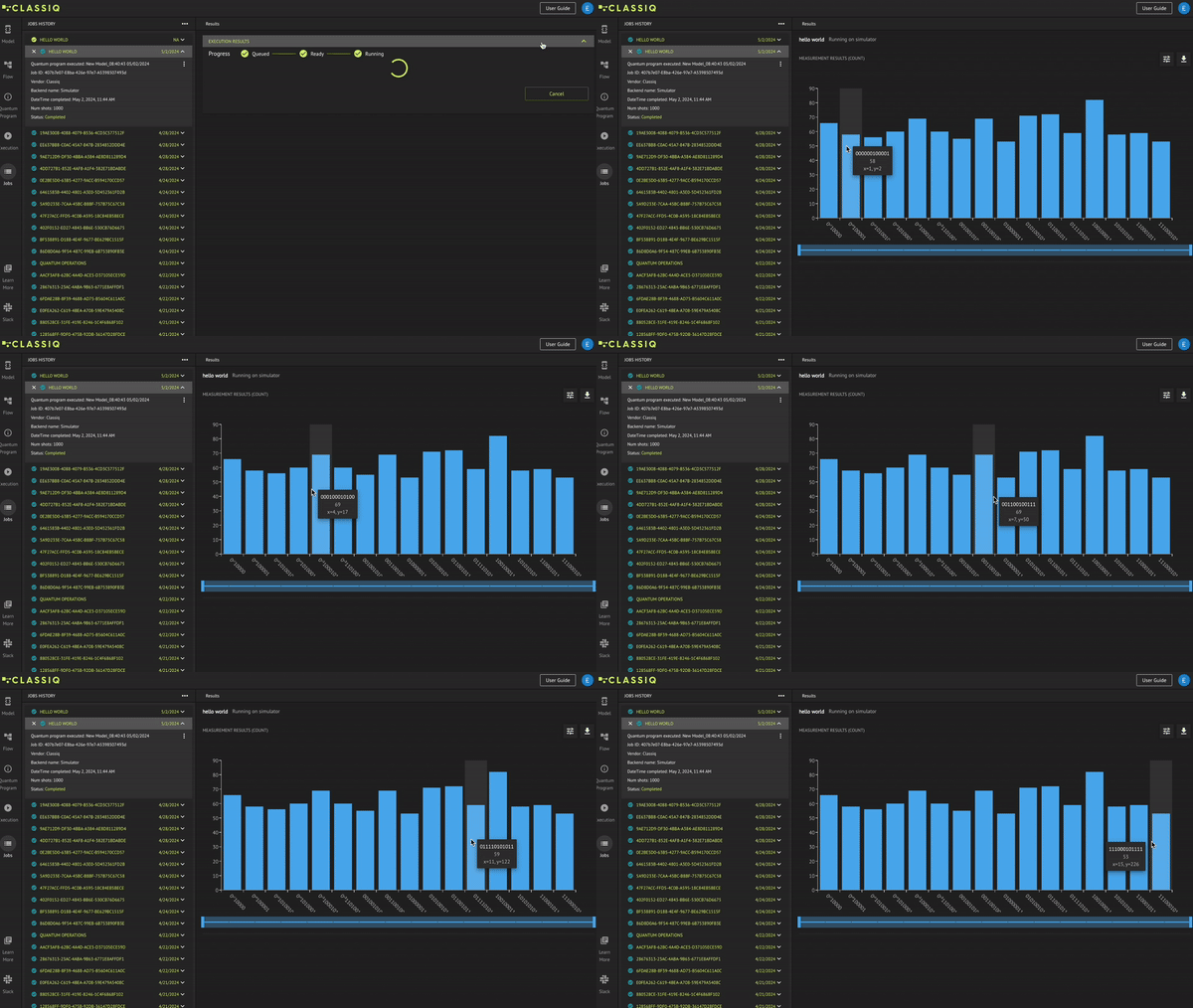
In the Jobs tab, check the results by hovering over the histogram bars and verifying you receive 16 bars. Each bar encapsulates the correct relation between \(x\) and \(y\); i.e., \(y=x^2+1\):
That's it! You just completed designing, optimizing, analyzing, and executing your first quantum algorithm with the Classiq IDE.
Design (SDK) - Optimize (SDK) - Analyze (IDE) - Execute (SDK)
Design your hello world quantum algorithm by running the following code in your favorite Python SDK environment (after installing Classiq):
from classiq import *


@qfunc
def main(x: Output[QNum], y: Output[QNum]):
    allocate(4, x)
    hadamard_transform(x)  # creates a uniform superposition
    y |= x**2 + 1
Optimize your algorithm by running this code from the Python SDK:
qprog_1 = synthesize(main)
Analyze your quantum circuit in the IDE by running this code in Python and opening the pop-up link:
show(qprog_1)
Opening: https://platform.classiq.io/circuit/2uG1nYzA9dUoa9icpRs44Mp5gNd?version=0.70.0

Execute your code in the Python SDK by running this:
results = execute(qprog_1).result_value()
print(results.parsed_counts)
[{'x': 6, 'y': 37}: 155, {'x': 8, 'y': 65}: 144, {'x': 13, 'y': 170}: 144, {'x': 11, 'y': 122}: 143, {'x': 5, 'y': 26}: 133, {'x': 12, 'y': 145}: 130, {'x': 9, 'y': 82}: 129, {'x': 7, 'y': 50}: 128, {'x': 2, 'y': 5}: 125, {'x': 4, 'y': 17}: 123, {'x': 3, 'y': 10}: 122, {'x': 0, 'y': 1}: 120, {'x': 14, 'y': 197}: 115, {'x': 1, 'y': 2}: 113, {'x': 10, 'y': 101}: 113, {'x': 15, 'y': 226}: 111]
Check that you receive 16 pairs of {'x': , 'y': } and that the values indeed follow the connection \(y=x^2+1\).
That's it! You just completed your first quantum algorithm in the Python SDK.
Design (SDK) - Optimize (SDK) - Analyze (IDE) - Execute (IDE)
Now, run the same example using a mixed flow of the previous two:
Design your hello world quantum algorithm by running this code in your favorite Python SDK environment (after installing Classiq):
from classiq import *


@qfunc
def main(x: Output[QNum], y: Output[QNum]):
    allocate(4, x)
    hadamard_transform(x)  # creates a uniform superposition
    y |= x**2 + 1
Optimize your algorithm by running this code in the Python SDK:
qprog_2 = synthesize(main)
Analyze your quantum circuit in the IDE by running this code in Python and opening the pop-up link:
show(qprog_2)
Opening: https://platform.classiq.io/circuit/2uG1ohlk2JsaupooIjMUCYNBaRL?version=0.70.0

Check that you receive two blocks in the quantum circuit: hadamard_transform and Arithmetic, then click Execute:

In the Execution tab, under the Classiq provider, choose the simulator (and make sure that other options are not selected). Change the job name to 'hello world' and click Run:

In the Jobs tab, check the results by hovering over the histogram bars and verifying you receive 16 bars. Each bar encapsulates the correct relation between \(x\) and \(y\); i.e., \(y=x^2+1\):

That's it! You just completed the hello world example in a mixed flow of IDE and Python SDK.
You are ready to continue with Classiq 101. Enjoy!
qmod = create_model(main, out_file="hello_many_worlds")