Quantum walk on complex network

View on GitHub

Open this notebook in GitHub to run it yourself

What this notebook does

Quantum walks are often used as building blocks for graph exploration / graph-based quantum algorithms. This notebook simulates a discrete-time quantum walk on a complex network (graph).

The graph is a set of nodes connected by edges (we generate it with NetworkX).
The walker position is stored in a quantum register x.
A second register y acts like a coin / direction / neighbor-choice register.
Each step of the walk applies:

Coin operator (mix amplitudes in a way that depends on the current node’s neighbors)
Shift operator (moves the walker according to the coin register)

At the end we measure the position register and plot a probability distribution over nodes.

Note: This is a discrete-time walk (coin + shift), not a continuous-time walk.

Imports and dependencies

import matplotlib.pyplot as plt
import networkx as nx
import numpy as np

from classiq import *

Step 1 — Create a “complex network” (the graph)

Here we generate a small graph G. The notebook currently uses a Watts–Strogatz model, which is a classic “small-world” network model:

it has high clustering (like regular lattices),
and short path lengths (like random graphs).

You can switch to other models by uncommenting the alternatives:

Erdős–Rényi (random graph)
Barabási–Albert (scale-free graph)

Then we draw the graph so we can visually connect the output distribution to the network structure.

G = nx.connected_watts_strogatz_graph(n=4, k=2, p=0.2, tries=100, seed=312)
# G = nx.erdos_renyi_graph(n=4, p=0.3, seed=42)
# G = nx.barabasi_albert_graph(n=8,m=2)
plt.figure(figsize=(3, 3))
nx.draw(
    G,
    with_labels=True,
    node_color="darkblue",
    edge_color="black",
    font_color="white",
    font_size=10,
)

Step 2 — Decide how many qubits are needed for the position register

If the graph has N nodes, we need enough qubits to encode node indices in binary.

N = len(G.nodes())
num_qubits = ceil(log2(N))

That means the quantum register x can represent 2**num_qubits = N.

N = len(G.nodes())
num_qubits = int(np.ceil(np.log2(N)))
print("number of nodes=", N, "number of required qubits=", num_qubits)

Output:

number of nodes= 4 number of required qubits= 2

Step 3 — Build “neighbor-aware” probability vectors

A quantum walk on a graph needs a way to represent “where can I go next from node

i

?”. We create helper functions:

get_edges_of_node(G, i): returns the neighbors of node i.
inner_degree(G, num_qubits, i): builds a length 2**num_qubits vector where:
- entries corresponding to neighbors of i are 1,
- all others are 0,
- then we normalize by the node degree k to get a uniform distribution over neighbors.

This vector is used to prepare the y register so it represents “allowed moves” from the current node.

def get_edges_of_node(G, i):
    return [j for j in G.neighbors(i)]


# DEGREE_LIST = np.zeros(N)
# for i in range(N):
#    DEGREE_LIST[i] = len(get_edges_of_node(G, i))


def inner_degree(G, num_qubits, i):
    l_array = np.zeros(2**num_qubits)
    neighbors_list = get_edges_of_node(G, i)
    k = len(neighbors_list)
    for j in neighbors_list:
        l_array[j] = 1
    return l_array / k

Step 4 — Define the quantum walk (state prep, coin, shift, and repeated steps)

This cell defines the core quantum logic using Classiq @qfunc.

Registers

x: position register (which node the walker is on)
y: coin / neighbor register (encodes the neighbor-choice space)

4.1 Initial state: `prepare_initial_state(x, y)`

Goal: start with a clean, interpretable state.

Prepare x in a uniform superposition over valid nodes:

If N is exactly 2**num_qubits, a Hadamard transform gives uniform superposition automatically.
Otherwise, we prepare a custom probability vector that gives equal weight to nodes 0..N-1 and zero to invalid states.

Prepare y conditioned on the current node in x: For each node i, if x == i, we prepare y using the neighbor distribution vector from inner_degree(...).

So after this, the state is conceptually:

“uniform over nodes” in x,
and for each node, y contains amplitudes only on its neighbors.

4.2 Coin operator: `my_coin(x, y)`

A discrete-time quantum walk needs a “coin flip” to mix amplitudes. Here, the coin depends on the current node:

If x == i, apply a Grover diffuser on register y corresponding to neighbors of node i.

This mixes the neighbor amplitudes in a structured way.

4.3 Shift operator: `my_shift(x, y)`

This updates the position based on the coin information.

4.4 Repeating steps: `discrete_quantum_walk(time, coin, shift, x, y)`

We apply the pair (coin, shift) repeatedly time times using power(time, ...). That is exactly the discrete-time walk loop: (coin → shift) × t

@qfunc
def prepare_initial_state(x: QNum[num_qubits], y: QNum[num_qubits]):
    if N == 2**num_qubits:
        hadamard_transform(x)
    else:
        prob_array = np.ones(2**num_qubits) / N
        prob_array[N : 2**num_qubits] = 0
        inplace_prepare_state(prob_array.tolist(), 0.0, x)
    for i in range(N):
        control(
            x == i,
            lambda: inplace_prepare_state(
                inner_degree(G, num_qubits, i).tolist(), 0.0, y
            ),
        )


@qfunc
def my_coin(x: QNum[num_qubits], y: QNum[num_qubits]):
    for i in range(N):
        control(
            x == i,
            stmt_block=lambda: grover_diffuser(
                lambda y: inplace_prepare_state(
                    inner_degree(G, num_qubits, i).tolist(), 0.0, y
                ),
                y,
            ),
        )


@qfunc
def my_shift(x: QNum[num_qubits], y: QNum[num_qubits]):
    multiswap(x, y)


@qfunc
def discrete_quantum_walk(
    time: CInt,
    coin_qfuncs: QCallable[QNum, QNum],
    shift_qfuncs: QCallable[QNum, QNum],
    x: QNum,
    y: QNum,
):
    power(
        time,
        lambda: (
            coin_qfuncs(x, y),
            shift_qfuncs(x, y),
        ),
    )

Step 5 — Choose number of steps, build `main`, and synthesize the circuit

Number of steps

t controls how far the quantum walk evolves. More steps usually means:

wider spreading over the graph,
more interference patterns,
sometimes more “structure” in the final distribution (depending on the graph).

The `main` quantum program

main(x: Output[QNum[num_qubits]]):

Allocates x (position) and y (coin).
Prepares the initial state.
Applies the discrete-time quantum walk for t steps.
Drops y (we only care about measuring the position distribution in x).

Finally:

synthesize(main) compiles the high-level program into an executable quantum program.
show(qprog) displays the synthesized result.

# quantum walk steps
t = 3


@qfunc
def main(x: Output[QNum[num_qubits]]):
    y = QNum("y", num_qubits)
    allocate(num_qubits, x)
    allocate(num_qubits, y)
    prepare_initial_state(x, y)
    discrete_quantum_walk(t, my_coin, my_shift, x, y)
    drop(y)


qprog = synthesize(main)
show(qprog)

Output:

Quantum program link: https://platform.classiq.io/circuit/3AYfsuRGxfFQPTvOVlovit1v2zJ
  

Output:

https://platform.classiq.io/circuit/3AYfsuRGxfFQPTvOVlovit1v2zJ?login=True&version=17
  

Step 6 — Execute and collect results

Here we run the synthesized program and fetch the results. The key output we care about is the measured distribution of the position register x:

each possible node index x has a probability,
these probabilities should sum to ~1 (up to sampling / execution effects).

execution_job = execute(qprog)
result = execution_job.result_value()

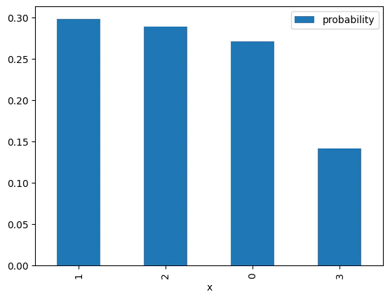
Step 7 — Visualize the probability distribution over nodes

We plot a bar chart:

x-axis: node index (the measured value of the position register x)
y-axis: probability of measuring that node

Tip for interpretation:

Compare “high-probability nodes” to the graph drawing.
Try changing the graph model or t and see how the distribution changes.

result.dataframe.plot.bar(x="x", y="probability")

Output:

<Axes: xlabel='x'>

(Optional) Hardware-Aware Synthesis and Hardware Execution

In this notebook, we executed the circuit on the ibm_torino processor. The Classiq platform allows specifying a particular processor through ExecutionPreferences. Before executing on quantum hardware, you can perform synthesis that incorporates hardware-specific constraints by configuring the preference settings. The following command runs hardware-aware synthesis to optimize your circuit for a target device. For more details, refer to the Hardware-Aware Synthesis.

# preferences = Preferences(
#     backend_service_provider="IBM Quantum", backend_name="ibm_torino"
# )
# synthesize(main, preferences=preferences)
# qprog = synthesize(main)

Once the synthesis is complete, you can configure the execution settings to run your circuit on a real quantum device or a specific simulator. The ExecutionPreferences class allows you to define parameters such as the number of shots and backend-specific credentials. The following code demonstrates how to set up an execution session for an IBM Quantum backend:

# execution_preferences = ExecutionPreferences(
#     num_shots=1024,
#     backend_preferences=IBMBackendPreferences(
#         backend_name='ibm_torino',
#         access_token="A Valid API access token to IBM Quantum",
#         channel="IBM Cloud Channel",
#         instance_crn="IBM Cloud Instance CRN",
#     )
# )

# with ExecutionSession(qprog, execution_preferences=execution_preferences) as es:
#     res = es.sample()

Result

$N=4$

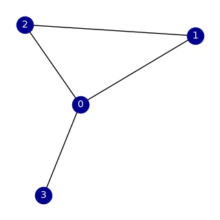
Once the graph structure is defined, you can perform a quantum spatial search to find a specific node. In this example, the search is conducted on a Watts-Strogatz small-world graph, which is generated using the NetworkX library to create a complex network topology. Below data is quantum spatial search on G = nx.connected_watts_strogatz_graph(n=4, k=2, p=0.2, tries=100, seed=312) .

import numpy as np

# withou HW synthesis
prob_torino_t1 = np.array([3258, 2340, 2549, 1853]) / 10000
prob_torino_t2 = np.array([2856, 2736, 2153, 2255]) / 10000
prob_torino_t3 = np.array([2474, 2468, 2389, 2669]) / 10000
prob_torino_t4 = np.array([2352, 2717, 2296, 2635]) / 10000

# with HW-level synthesis
prob_torino_t1_hw = np.array([2228, 2650, 2286, 2836]) / 10000
prob_torino_t2_hw = np.array([2296, 2428, 2461, 2815]) / 10000
prob_torino_t3_hw = np.array([2567, 2477, 2483, 2473]) / 10000
prob_torino_t4_hw = np.array([2269, 2385, 2339, 3007]) / 10000

# Simulator result (ideal)
prob_sim_t1 = [0.5, 0.20833333, 0.20833333, 0.08333333]
prob_sim_t2 = [0.33333333, 0.28690075, 0.28690075, 0.09286516]
prob_sim_t3 = [0.25953183, 0.29985427, 0.29985427, 0.14075964]
prob_sim_t4 = [0.54789448, 0.1859174, 0.1859174, 0.08027073]

prob_torino_list_n4 = [prob_torino_t1, prob_torino_t2, prob_torino_t3, prob_torino_t4]
prob_torino_hw_list_n4 = [
    prob_torino_t1_hw,
    prob_torino_t2_hw,
    prob_torino_t3_hw,
    prob_torino_t4_hw,
]
prob_sim_list_n4 = [prob_sim_t1, prob_sim_t2, prob_sim_t3, prob_sim_t4]

$N=8$

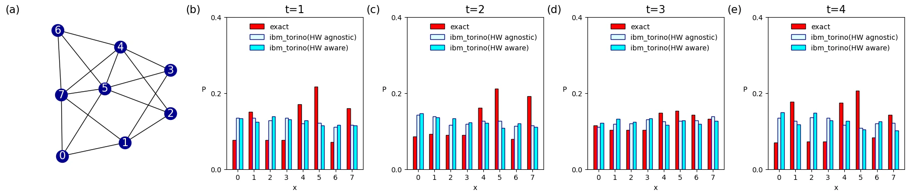
Below data is quantum spatial search on G = nx.connected_watts_strogatz_graph(n=8, k=4, p=0.2, tries=100, seed=312) .

# withou HW synthesis
prob_torino_t1 = np.array([1330, 1238, 1391, 1302, 1283, 1144, 1158, 1154]) / 10000
prob_torino_t2 = np.array([1463, 1361, 1340, 1230, 1214, 1083, 1202, 1107]) / 10000
prob_torino_t3 = np.array([1213, 1320, 1243, 1334, 1160, 1277, 1183, 1270]) / 10000
prob_torino_t4 = np.array([1487, 1175, 1478, 1276, 1272, 1038, 1258, 1016]) / 10000

# with HW-level synthesis
prob_torino_t1_hw = np.array([1350, 1352, 1275, 1342, 1205, 1214, 1104, 1158]) / 10000
prob_torino_t2_hw = np.array([1431, 1386, 1167, 1187, 1274, 1273, 1135, 1147]) / 10000
prob_torino_t3_hw = np.array([1115, 1186, 1195, 1306, 1250, 1274, 1283, 1391]) / 10000
prob_torino_t4_hw = np.array([1347, 1270, 1363, 1351, 1167, 1087, 1201, 1214]) / 10000

# Simulator result (ideal)
prob_sim_t1 = [
    0.07708333,
    0.15,
    0.07708333,
    0.07708333,
    0.17083333,
    0.21666667,
    0.07083333,
    0.16041667,
]
prob_sim_t2 = [
    0.0856499,
    0.09285754,
    0.08907021,
    0.08907021,
    0.16118512,
    0.21198126,
    0.07902679,
    0.19115897,
]
prob_sim_t3 = [
    0.11548278,
    0.10271175,
    0.10264854,
    0.10264854,
    0.14767895,
    0.15389152,
    0.14311526,
    0.13182268,
]
prob_sim_t4 = [
    0.06987609,
    0.17753849,
    0.072522,
    0.072522,
    0.17425693,
    0.20675877,
    0.08323824,
    0.14328747,
]

prob_torino_list_n8 = [prob_torino_t1, prob_torino_t2, prob_torino_t3, prob_torino_t4]
prob_torino_hw_list_n8 = [
    prob_torino_t1_hw,
    prob_torino_t2_hw,
    prob_torino_t3_hw,
    prob_torino_t4_hw,
]
prob_sim_list_n8 = [prob_sim_t1, prob_sim_t2, prob_sim_t3, prob_sim_t4]

Vizualization

import matplotlib.pyplot as plt
import networkx as nx
import numpy as np

G = nx.connected_watts_strogatz_graph(n=8, k=4, p=0.2, tries=100, seed=312)

x = np.arange(8)
width = 0.2
gap = 0.4
titles = ["t=1", "t=2", "t=3", "t=4"]

fig, axes = plt.subplots(1, 5, figsize=(18, 4))
axes = axes.flatten()


panel_labels = ["(a)", "(b)", "(c)", "(d)", "(e)"]
ax0 = axes[0]
pos = nx.spring_layout(G, seed=312)

nx.draw(
    G,
    pos=pos,
    ax=ax0,
    with_labels=True,
    node_color="darkblue",
    edge_color="black",
    font_color="white",
    font_size=15,
)

ax0.text(-0.3, 1.08, panel_labels[0], transform=ax0.transAxes, fontsize=15, va="top")

prob_sim_list = prob_sim_list_n8
prob_torino_list = prob_torino_hw_list_n8
prob_torino_hw_list = prob_torino_list_n8

for i in range(4):
    ax = axes[i + 1]

    ax.bar(
        x - gap / 2,
        prob_sim_list[i],
        width=width,
        color="red",
        edgecolor="black",
        label="exact",
    )
    ax.bar(
        x,
        prob_torino_list[i],
        width=width,
        color="lightcyan",
        edgecolor="darkblue",
        label="ibm_torino(HW agnostic)",
    )
    ax.bar(
        x + gap / 2,
        prob_torino_hw_list[i],
        width=width,
        color="cyan",
        edgecolor="darkblue",
        label="ibm_torino(HW aware)",
    )

    ax.set_title(titles[i], fontsize=15)
    ax.set_ylabel("P", rotation=0, labelpad=10)
    ax.set_xlabel("x")
    ax.set_ylim(0, 0.3)
    ax.set_xticks(x)
    ax.set_yticks([0.0, 0.2, 0.4])
    ax.legend(fontsize=10, frameon=False)
    ax.text(
        -0.3, 1.08, panel_labels[i + 1], transform=ax.transAxes, fontsize=15, va="top"
    )

plt.tight_layout()
plt.show()

Algorithms

Applications

Functions

Tutorials

Quantum walk on complex network

View on GitHub

What this notebook does

Imports and dependencies

Step 1 — Create a “complex network” (the graph)

Step 2 — Decide how many qubits are needed for the position register

Step 3 — Build “neighbor-aware” probability vectors

Step 4 — Define the quantum walk (state prep, coin, shift, and repeated steps)

Registers

4.1 Initial state: `prepare_initial_state(x, y)`

4.2 Coin operator: `my_coin(x, y)`

4.3 Shift operator: `my_shift(x, y)`

4.4 Repeating steps: `discrete_quantum_walk(time, coin, shift, x, y)`

Step 5 — Choose number of steps, build `main`, and synthesize the circuit

Number of steps

The `main` quantum program

Step 6 — Execute and collect results

Step 7 — Visualize the probability distribution over nodes

(Optional) Hardware-Aware Synthesis and Hardware Execution

Result

$N=4$

$N=8$

Vizualization

Algorithms

Applications

Functions

Tutorials

View on GitHub

​What this notebook does

​Imports and dependencies

​Step 1 — Create a “complex network” (the graph)

​Step 2 — Decide how many qubits are needed for the position register

​Step 3 — Build “neighbor-aware” probability vectors

​Step 4 — Define the quantum walk (state prep, coin, shift, and repeated steps)

​

​Registers

​

​4.1 Initial state: prepare_initial_state(x, y)

​

​4.2 Coin operator: my_coin(x, y)

​

​4.3 Shift operator: my_shift(x, y)

​

​4.4 Repeating steps: discrete_quantum_walk(time, coin, shift, x, y)

​Step 5 — Choose number of steps, build main, and synthesize the circuit

​

​Number of steps

​

​The main quantum program

​Step 6 — Execute and collect results

​Step 7 — Visualize the probability distribution over nodes

​(Optional) Hardware-Aware Synthesis and Hardware Execution

​Result

​N=4N=4N=4

​N=8N=8N=8

​Vizualization

What this notebook does

Imports and dependencies

Step 1 — Create a “complex network” (the graph)

Step 2 — Decide how many qubits are needed for the position register

Step 3 — Build “neighbor-aware” probability vectors

Step 4 — Define the quantum walk (state prep, coin, shift, and repeated steps)

Registers

4.1 Initial state: `prepare_initial_state(x, y)`

4.2 Coin operator: `my_coin(x, y)`

4.3 Shift operator: `my_shift(x, y)`

4.4 Repeating steps: `discrete_quantum_walk(time, coin, shift, x, y)`

Step 5 — Choose number of steps, build `main`, and synthesize the circuit

Number of steps

The `main` quantum program

Step 6 — Execute and collect results

Step 7 — Visualize the probability distribution over nodes

(Optional) Hardware-Aware Synthesis and Hardware Execution

Result

$N=4$

$N=8$

Vizualization