
View on GitHub

Open this notebook in GitHub to run it yourself
Quantum computing is based on the principles of quantum mechanics, which includes an important feature: unitarity. The operations that evolve quantum states on quantum computers are unitary. Would this mean that problems requiring non-unitary operations are out of hand for quantum computers? This is the task solved by the Linear Combination of Unitaries (LCU) algorithm [1, 2]. Given a non-unitary matrix AA that can be decomposed into a sum of unitary matrices as follows: A=i=02n1αiUi,\begin{equation} A = \sum_{i=0}^{2^n-1} \alpha_i U_i, \end{equation} where αi\alpha_i are real, positive coefficients and UiU_i are unitary matrices, the LCU algorithm applies the action of AA, up to a normalization factor, on a desired quantum state. It does so by embedding the matrix AA in a bigger unitary. The first step of the LCU is to prepare the following state on an auxiliary quantum register according to the coefficients αi\alpha_i using the function PREPARE: ψ0=PREPARE0=iαiλi,\begin{equation} |\psi_0\rangle = PREPARE|0\rangle = \sum_i \sqrt{\frac{\alpha_i}{\lambda}}|i\rangle, \end{equation} where λ=iαi\lambda = \sum_i |\alpha_i| is a normalization factor. This quantum register with the prepared state is used as a controller for the next step. Then, according to the controller quantum register, the following state is being prepared: SELECTiψ=iUiψ,\begin{equation} SELECT|i\rangle|\psi\rangle = |i\rangle U_i |\psi\rangle, \end{equation} where ψ|\psi\rangle is the desired quantum state the matrix AA should be applied on. The final step is to have the PREPARE operation inversed such that the following desired state is created: LCU0ψ=PREPARE1SELECTPREPARE0ψ=V0ψ,\begin{equation} LCU|0\rangle|\psi\rangle = PREPARE^{-1}\, SELECT\, PREPARE |0\rangle|\psi\rangle = V |0\rangle |\psi\rangle, \end{equation} where VV can be represented as V=[A].V = \begin{bmatrix}A & \cdot \\ \cdot & \cdot \end{bmatrix}. This is called the Block Encoding of the matrix A. By projecting the controller quantum register on the 0|0\rangle state the desired outcome is obtained: (00I)LCU0ϕ=0Aλψ.\begin{equation} \left(|0\rangle\langle0|\otimes I\right)LCU|0\rangle|\phi\rangle = |0\rangle\frac{A}{\lambda}|\psi\rangle. \end{equation} Therefore, the action of the sequence of operations over the target qubit will be the non-unitary operation AA, up to a normalization factor. A detailed mathematical description of the algorithm can be seen below and in reference [1]. It is also important to notice that the projection onto the 0|0\rangle state depends on a success probability, detailed in [1]. Overall, a scheme of the algorithm looks like:

Guided Implementation

Now that we know how the LCU algorithm works, it’s time to implement it on Classiq. For that, we will be using two important functions:
The Within-Apply maps unitary operations of the kind V=U1WUV = U^{-1}WU into the quantum circuit, given UU and WW.
The Prepare state function realizes the initial state preparation step of a quantum algorithm, given a bound for the error and the probabilities of the quantum states. Using this tutorial, one can play with this function. The objective of our quantum circuit is to define the matrices UU and WW following the V=U1WUV = U^{-1} W U decomposition used in the Within-Apply function. A quick look on the definition of the LCU operator is enough to identify U=PREPAREU = PREPARE and W=SELECTW = SELECT. As an example, we will be considering the following SELECT operator: SELECT=00I+11QFT+22QFT1,\begin{equation} SELECT = |0\rangle\langle 0|\otimes I + |1\rangle\langle 1|\otimes QFT + |2\rangle\langle 2| \otimes QFT^{-1}, \end{equation} where QFT is the Quantum Fourier Transform operator that acts over the two target qubits, and that the probabilities are α=[0.5,0.25,0.25,0]\alpha = [0.5,0.25,0.25,0]. Now that the operations are identified, we just need to build them and then use the Within-Apply function. The SELECT operation can be build using the control statement, and the QFT function:
from classiq import *


@qfunc
def select(controller: QNum, psi: QNum):
    control(ctrl=controller == 0, stmt_block=lambda: apply_to_all(IDENTITY, psi))

    control(ctrl=controller == 1, stmt_block=lambda: qft(psi))

    control(ctrl=controller == 2, stmt_block=lambda: invert(lambda: qft(psi)))
Using two auxiliary qubits, this sequence of operations can be seen in Classiq’s IDE as select.gif 
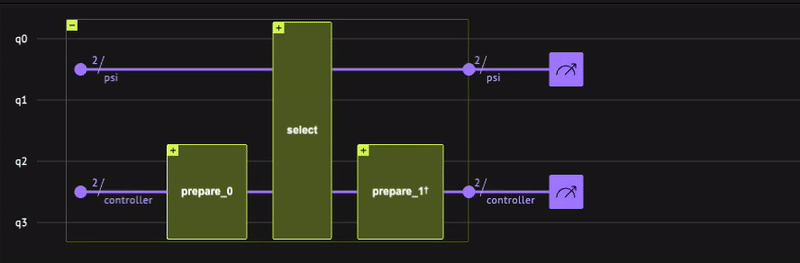
With the SELECT function defined, we are able to apply the V operator, by using the Within-Apply function. For this, it is necessary to build the PREPARE operator, which will be done using the inplace_prepare_state() function, that requires the probability distribution α\alpha, the maximum error in the decomposition of the operator and the target qubits, which are the controllers.
@qfunc
def prepare(controller: QNum):
    # Defining the error bound and probability distribution
    error_bound = 0.01
    controller_probabilities = [0.5, 0.25, 0.25, 0]
    inplace_prepare_state(controller_probabilities, error_bound, controller)
Thus, the sequence of operations we will define in our quantum program is:
  • Define the error bound in the decomposition, and define the probability distribution α\alpha
  • Allocate target and control qubits
  • Execute the Within-Apply function, using the PREPARE and SELECT functions
@qfunc
def main(controller: Output[QNum], psi: Output[QNum]):
    # Allocating the target and control qubits, respectively
    allocate(2, psi)
    allocate(2, controller)
    # Executing the Within-Apply function with the select and the prepare functions.
    within_apply(
        within=lambda: prepare(controller),
        apply=lambda: select(controller, psi),
    )


qmod_1 = create_model(main)
qprog_1 = synthesize(qmod_1)
Your quantum program is done! You can see it using Classiq’s IDE with the show() command:
show(qprog_1)
Output:

Quantum program link: https://platform.classiq.io/circuit/39FkkG2O0kmXD4dTWHX7WKDCm4r
  

Output:
https://platform.classiq.io/circuit/39FkkG2O0kmXD4dTWHX7WKDCm4r?login=True&version=17
  

Mathematical Description

The initial state of our circuit is 0Ψ|0\rangle|\Psi\rangle, for some general Ψ\Psi. After that, the PREPARE operation is applied, transforming it in the state: PREPARE0Ψ=(i=02n1αiλi)Ψ.\begin{equation} PREPARE|0\rangle|\Psi\rangle = \left(\sum_{i=0}^{2^n-1} \sqrt{\frac{|\alpha_i|}{\lambda}} |i\rangle\right)|\Psi\rangle. \end{equation} We can always represent the PREPARE operation, which acts only in the control qubits, as being: PREPARE=i=02n1αiλi0+i=02n1j=12n1βi,jij,\begin{equation} PREPARE = \sum_{i=0}^{2^n-1} \sqrt{\frac{|\alpha_i|}{\lambda}} |i\rangle\langle 0| + \sum_{i=0}^{2^n-1}\sum_{j=1}^{2^n-1} \beta_{i,j} |i\rangle\langle j|, \end{equation} for some βi,j\beta_{i,j}. The SELECT operation, which acts both in the control and target qubits, can also be described this way by SELECT=i=02n1iiUi.\begin{equation} SELECT = \sum_{i=0}^{2^n-1} |i\rangle\langle i|\otimes U_i. \end{equation} Now, the state generated by PREPARE1SELECTPREPARE0ψPREPARE^{-1}\, SELECT\, PREPARE |0\rangle|\psi\rangle is given by: PREPARE1SELECTPREPARE0ψ=1λ0i=02n1αiUiΨ+j=12n1(i=02n1βi,j)jUjΨ\begin{equation} PREPARE^{-1}\, SELECT\, PREPARE |0\rangle|\psi\rangle = \frac{1}{\lambda}|0\rangle\sum_{i=0}^{2^n-1} \alpha_i \, U_i |\Psi\rangle + \sum_{j=1}^{2^n-1} \left( \sum_{i=0}^{2^n-1} \beta_{i,j}^*\right) |j\rangle\,U_j |\Psi\rangle \end{equation} When applying the projector 00|0\rangle\langle 0| onto the control qubits, we finally obtain the desired state 1λ0i=02n1αiUiΨ=0AλΨ.\begin{equation} \frac{1}{\lambda}|0\rangle\sum_{i=0}^{2^n-1} \alpha_i \, U_i |\Psi\rangle = |0\rangle\frac{A}{\lambda}|\Psi\rangle. \end{equation}

All the Code Together

from classiq import *


@qfunc
def select(controller: QNum, psi: QNum):
    control(ctrl=controller == 0, stmt_block=lambda: apply_to_all(IDENTITY, psi))

    control(ctrl=controller == 1, stmt_block=lambda: qft(psi))

    control(ctrl=controller == 2, stmt_block=lambda: invert(lambda: qft(psi)))


@qfunc
def prepare(controller: QNum):
    # Defining the error bound and probability distribution
    error_bound = 0.01
    controller_probabilities = [0.5, 0.25, 0.25, 0]
    inplace_prepare_state(controller_probabilities, error_bound, controller)


@qfunc
def main(controller: Output[QNum], psi: Output[QNum]):
    # Allocating the target and control qubits, respectively
    allocate(2, psi)
    allocate(2, controller)
    # Executing the Within-Apply function with the select and the prepare functions.
    within_apply(
        within=lambda: prepare(controller),
        apply=lambda: select(controller, psi),
    )


qmod_2 = create_model(main)
qprog_2 = synthesize(qmod_2)

show(qprog_2)
Output:

Quantum program link: https://platform.classiq.io/circuit/39FklKFg3swhJR0OH8xkqcRIWqb
  

Output:
https://platform.classiq.io/circuit/39FklKFg3swhJR0OH8xkqcRIWqb?login=True&version=17
  

References

[1]: Hamiltonian Simulation Using Linear Combinations of Unitary Operations (Andrew M. Childs and Nathan Wiebe) [2]: Lecture Notes on Quantum Algorithms (Andrew M. Childs)