View on GitHub

Open this notebook in GitHub to run it yourself

The notebook demonstrates the solution of a generic optimization problem using both the “vanilla” QAOA (Quantum Approximate Optimization Algorithm) and the adaptive version

Hamiltonian encoding

The optimization objective function is encoded into a Hamiltonian function formulated as a weighted sum of Pauli strings:

H = \sum_k{c_kP_k}

with each pauli string,

P_k

, composed of a Pauli operation (

\sigma\in\left\{I,X,Y,Z\right\}

) applied to each of the qubits in the register. For example,

XIIZ

, applies a Pauli

X

to the first qubit and a Pauli

Z

to the fourth qubit The encoding of the objective start by defining the function with binary variables,

x_i\in\left\{1,-1\right\}

, and then defining Pauli strings with

Z_i

corresponding to the original variables. If the objective variables’ domain is

x_i\in\left\{0,1\right\}

, a transformation is used:

x_i=\left(1-Z_i\right)/2

(commonly referred to as spin to bit transformation) Since the encoding results in Pauli strings composed only of

I

, and

Z

, the Pauli string is called diagonal, this has the following benefits:

Easy exponentiation - the exponentiation results in simple to implement single or multi-qubit Z rotations
No superposition mixing - the diagonal Hamiltonian does not create entanglement or rotate between basis states, enabling computation basis measurement
Efficient measurement - all $\left\{I,Z\right\}^{\otimes n}$ strings commute, allowing for a single simultaneous measurement of all strings

import matplotlib.pyplot as plt
import numpy as np
import scipy
from tqdm import tqdm

from classiq import *

QMod tip

In the following cell the variable h is set to a diagonal hamiltonian using a self explanatory syntax that sums sparse Pauli strings, that is only the non identity Paulis are specified. For example the first line, - 0.1247375 * Pauli.Z(0) * Pauli.Z(1) creates the string ZZIII with the weight -0.1247375. The length of the string, is inferred from the largest qubit index in the sum. The resulating variable has the type SparsePauliOp For the optimization function a dual-use function is used for the Hamiltonian. This function takes a argument that can be either a QArray or a list[int]. This allows the same function to be used both to:

compute the cost expectation on the measurement results which are binary numbers ( $0,1$ )
create a quantum observable in the circuit, resulting in quantum gates

the additional cost_func function negates the hamiltonian function since the problem involves finding the maximum value, but the optimization procedure (scipy.optimize.minimize) performs a minimization

from typing import Tuple

from sympy import sympify

from classiq import IndexedPauli, Pauli, SparsePauliOp, SparsePauliTerm
from classiq.qmod.symbolic_expr import SymbolicExpr

QFloatExr = SymbolicExpr


h = (
    -0.561775 * Pauli.Z(0)
    - 1.238125 * Pauli.Z(1)
    - 1.131450 * Pauli.Z(2)
    - 0.681350 * Pauli.Z(3)
    - 0.713775 * Pauli.Z(4)
    - 0.979450 * Pauli.Z(5)
    - 1.145025 * Pauli.Z(6)
    - 0.774450 * Pauli.Z(7)
    + 0.5 * Pauli.Z(0) * Pauli.Z(1)
    + 0.5 * Pauli.Z(0) * Pauli.Z(2)
    - 0.188125 * Pauli.Z(0) * Pauli.Z(4)
    - 0.200100 * Pauli.Z(0) * Pauli.Z(5)
    + 0.5 * Pauli.Z(1) * Pauli.Z(3)
    + 0.234550 * Pauli.Z(1) * Pauli.Z(6)
    + 0.053575 * Pauli.Z(1) * Pauli.Z(7)
    + 0.5 * Pauli.Z(2) * Pauli.Z(3)
    - 0.048100 * Pauli.Z(2) * Pauli.Z(4)
    + 0.229550 * Pauli.Z(2) * Pauli.Z(5)
    - 0.039525 * Pauli.Z(3) * Pauli.Z(6)
    - 0.229125 * Pauli.Z(3) * Pauli.Z(7)
    + 0.5 * Pauli.Z(4) * Pauli.Z(5)
    + 0.5 * Pauli.Z(4) * Pauli.Z(6)
    + 0.5 * Pauli.Z(5) * Pauli.Z(7)
    + 0.5 * Pauli.Z(6) * Pauli.Z(7)
)


def hamiltonian(v: QArray | list[int]) -> QFloatExr:
    # linear Z_i coefficients (diagonal of hh)
    single_weights = [
        -0.561775,  # Z0
        -1.238125,  # Z1
        -1.13145,  # Z2
        -0.68135,  # Z3
        -0.713775,  # Z4
        -0.97945,  # Z5
        -1.145025,  # Z6
        -0.77445,  # Z7
    ]

    # quadratic ZZ coefficients (off-diagonal of hh for i<j)
    quadratic_pairs = [
        (0, 1),
        (0, 2),
        (0, 4),
        (0, 5),
        (1, 3),
        (1, 6),
        (1, 7),
        (2, 3),
        (2, 4),
        (2, 5),
        (3, 6),
        (3, 7),
        (4, 5),
        (4, 6),
        (5, 7),
        (6, 7),
    ]
    quadratic_weights = [
        0.5,
        0.5,
        -0.188125,
        -0.2001,
        0.5,
        0.23455,
        0.053575,
        0.5,
        -0.0481,
        0.22955,
        -0.039525,
        -0.229125,
        0.5,
        0.5,
        0.5,
        0.5,
    ]

    def z_value(bit: int | QBit) -> QFloatExr:
        # maps v_i in {0,1} to Z_i in {+1,-1}
        return sympify(1.0) - 2 * bit

    ham = sympify(0.0)  # no constant term in your SparsePauliOp

    # ZZ terms
    for (i, j), w in zip(quadratic_pairs, quadratic_weights):
        ham += w * z_value(v[i]) * z_value(v[j])

    # Z terms
    for i, w in enumerate(single_weights):
        ham += w * z_value(v[i])

    return ham


def cost_func(v: QArray | list[int]) -> QFloatExr:
    return hamiltonian(v)  # negative sign for maximization

The Cost Layer

As mentioned above, since the Hamiltonian is diagonal, its exponentiation is straightforward and amounts to phase addition due to Z rotations.
This is accomplished with the phase function, which results in an efficient quantum implementation of

e^{-i \gamma H_c}

@qfunc
def cost_layer(gamma: CReal, v: QArray):
    phase(cost_func(v), gamma)

The Mixer Layer

The QAOA mixer is defined as

H_M=\sum{X_i}

, and its exponentiaion is simply a

R_X

rotation of the same angle (

\beta

) on all the qubits

@qfunc
def mixer_layer(beta: CReal, qba: QArray):
    apply_to_all(lambda q: RX(2 * beta, q), qba)

The QAOA Ansatz

The parametric QAOA ansatz is composed of

p

pairs of exponentiated Mixer and Cost Hamiltonians:

U\left(\vec{\beta},\vec{\gamma}\right)=e^{-i \beta_p H_M}e^{-i \gamma_p H_C}\ldots e^{-i \beta_2 H_M}e^{-i \gamma_1 H_C}e^{-i \beta_2 H_M}e^{-i \gamma_1 H_C}

@qfunc
def qaoa_ansatz(
    gammas: CArray[CReal],
    betas: CArray[CReal],
    qba: QArray,
):
    n = gammas.len
    assert n == betas.len, "Number of gamma and beta parameters must be equal"
    for i in range(n):
        cost_layer(gammas[i], qba)
        mixer_layer(betas[i], qba)

Assemble the full QAOA algorithm

We select

p=3

layers for the QAOA. The quantum program takes the

2p

parameters as a single list (because the scipy.optimize.minimize function manipulate a 1-D array of parameters), and the quantum register of the

5

qubits. The qubits are initialized to

\left|+\right\rangle^{\otimes 5}

, with a hadamard_transform and then the qaoa_ansatz,

U\left(\vec{\beta},\vec{\gamma}\right)

, is applied

from typing import Final

NUM_LAYERS: Final[int] = 3
NUM_QUBITS: Final[int] = 8


@qfunc
def main(
    params: CArray[
        CReal, NUM_LAYERS * 2  # type: ignore
    ],  # Execution parameters (first half: gammas, second half: betas)
    v: Output[QArray[QBit, NUM_QUBITS]],  # type: ignore
):
    allocate(v)
    hadamard_transform(v)
    gammas = params[0:NUM_LAYERS]
    betas = params[NUM_LAYERS : NUM_LAYERS * 2]

    qaoa_ansatz(gammas, betas, v)

from classiq.execution.execution_session import ExecutionSession
from classiq.synthesis import show, synthesize

custom_hardware_settings = CustomHardwareSettings(basis_gates=["cz", "rz", "rx", "ry"])
#     connectivity_map = [
#     (0, 1), (1, 2), (2, 3),
#     (4, 5), (5, 6), (6, 7),
#     (0, 4), (1, 5), (2, 6), (3, 7)
# ],
#     is_symmetric_connectivity=True,
# )
preferences = Preferences(custom_hardware_settings=custom_hardware_settings)

qprog = synthesize(main, preferences=preferences)

es = ExecutionSession(qprog)
# show(qprog)

# circuit width
print(f"circuit width: {qprog.data.width}")
# circuit depth
print(f"circuit depth: {qprog.transpiled_circuit.depth}")

Output:

circuit width: 8
  circuit depth: 241
  

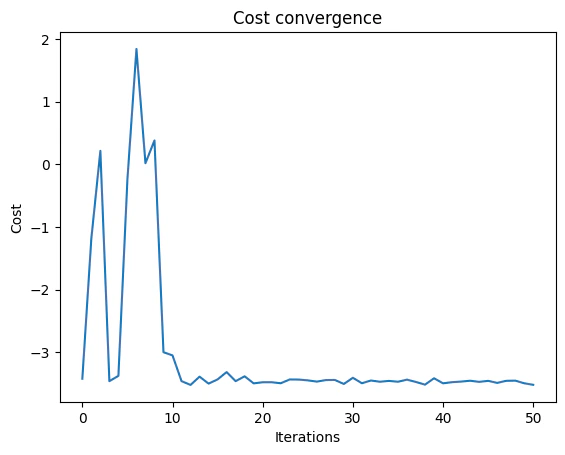
Classical Optimization - “Vanilla” QAOA

The

\vec{\beta}

, and

\vec{\gamma}

parameters are tuned until the objective function converges. The results of the parameters, and the solution vector are shown below

cost_trace = []
params_history = []


def objective_func(params, es):
    cost_estimation = es.estimate_cost(
        lambda state: cost_func(state["v"]), {"params": params.tolist()}
    )
    cost_trace.append(cost_estimation)
    params_history.append(params.copy())
    return cost_estimation

# TODO: uncomment
MAX_ITERATIONS = 60

initial_params = np.concatenate(
    (np.linspace(0, 1, NUM_LAYERS), np.linspace(1, 0, NUM_LAYERS))
)

with tqdm(total=MAX_ITERATIONS, desc="Optimization Progress", leave=True) as pbar:

    def progress_bar(xk: np.ndarray) -> None:
        pbar.update(1)

    obj = lambda params: objective_func(params, es)

    optimization_results = scipy.optimize.minimize(
        fun=obj,
        x0=initial_params,
        method="COBYLA",
        options={"maxiter": MAX_ITERATIONS},
        callback=progress_bar,
    )

# Sample the circuit using the optimized parameters
res = es.sample({"params": optimization_results.x.tolist()})
es.close()

print(f"Optimized parameters: {optimization_results.x.tolist()}")

Output:

Optimization Progress:  40%|███████████████████████████████▏                                              | 24/60 [01:26<02:10,  3.62s/it]
  

Output:

Optimized parameters: [0.023764076850575737, 0.4788895138030138, 1.999274060087544, 0.9995157762026724, 0.4815685457228382, 0.09300073147966786]
  

Plotting the convergence graph:

plt.plot(cost_trace)
plt.xlabel("Iterations")
plt.ylabel("Cost")
plt.title("Cost convergence")
plt.show()

Displaying and Discussing the Results

print(f"Optimized parameters: {optimization_results.x.tolist()}")
sorted_counts = sorted(res.parsed_counts, key=lambda pc: cost_func(pc.state["v"]))
num_shots = sum(state.shots for state in res.parsed_counts)
for sampled in sorted_counts[:10]:
    solution = sampled.state["v"]
    probability = sampled.shots / num_shots
    cost_value = cost_func(solution)
    print(f"solution={solution} probability={probability:.3f} cost={cost_value:.3f}")

Output:

Optimized parameters: [0.023764076850575737, 0.4788895138030138, 1.999274060087544, 0.9995157762026724, 0.4815685457228382, 0.09300073147966786]
  solution=[1, 0, 0, 1, 1, 0, 0, 1] probability=0.037 cost=-5.482
  solution=[1, 0, 0, 1, 0, 1, 1, 0] probability=0.012 cost=-4.771
  solution=[1, 0, 0, 1, 0, 0, 0, 1] probability=0.021 cost=-4.629
  solution=[0, 0, 0, 1, 1, 0, 0, 1] probability=0.014 cost=-4.629
  solution=[0, 0, 0, 1, 0, 0, 0, 1] probability=0.031 cost=-4.529
  solution=[1, 0, 0, 1, 0, 1, 0, 0] probability=0.026 cost=-4.513
  solution=[1, 0, 0, 0, 0, 1, 1, 0] probability=0.020 cost=-4.513
  solution=[1, 0, 0, 0, 1, 0, 0, 1] probability=0.017 cost=-4.465
  solution=[1, 0, 0, 1, 1, 0, 0, 0] probability=0.013 cost=-4.465
  solution=[1, 0, 0, 0, 0, 1, 0, 0] probability=0.042 cost=-4.413
  

ADAPT QAOA

The algorithm, based on the paper An adaptive quantum approximate optimization algorithm for solving combinatorial problems on a quantum computer, modifies QAOA by using different mixer layers, instead of the original

H_M=\sum_i{X_i}

. The algorithm defines a pool of potential mixer layers, that are simple to implement, and can match the problem better. The motiviation to the algorithm is rooted in t STA (shortcut to adiabaticity), with the hope of achieving better convergence than the “vanilla” QAOA. The algorithm proceeds incrementally:

initially, a single mixer layer is used (the original $H_M$ ) and the parameters are optimized
all the potential mixer layers, $A_j$ , are tested as candidates.

The criterion is the resulting gradient of the commutator of a potential mixer layer with the cost Hamiltonian, applied to the current circuit:

\nabla A_j = \left\langle\psi^{\left(k-1\right)}\right|e^{i \gamma_0 H_C}\left[H_C,A_j\right]e^{-i \gamma_0 H_C}\left|\psi^{\left(k-1\right)}\right\rangle

the mixer layer with the largest gradient is selected, the circuit grows by one layer, and the process continues (optimizing parameters and checking gradients)
the process terminates when the scaled norm of the gradient vector drops below a threshold

Utilities

The following functions define some convenience utilities for computing the commutation of Pauli strings

from functools import reduce
from operator import add, mul

# the following utilites are used to compute an expectation value of the form:
# <psi | [A,H] | psi>
# where psi is the state (ansatz), A and H are a mixer and cost Hamiltonians, respectively
# defined as pauli strings (SparsePauliOp)

# multiplication table of two Pauli matrices
# weight (imaginary), pauli_c = pauli_a * pauli_b
pauli_mult_table: list[list[Tuple[int, int]]] = [
    [(+0, Pauli.I), (+0, Pauli.X), (+0, Pauli.Y), (+0, Pauli.Z)],
    [(+0, Pauli.X), (+0, Pauli.I), (+1, Pauli.Z), (-1, Pauli.Y)],
    [(+0, Pauli.Y), (-1, Pauli.Z), (+0, Pauli.I), (+1, Pauli.X)],
    [(+0, Pauli.Z), (+1, Pauli.Y), (-1, Pauli.X), (+0, Pauli.I)],
]


def sorted_pauli_term(term: SparsePauliTerm) -> SparsePauliTerm:
    """
    sort pauli terms according to the qubit's index, e.g.,
    Pauli.X(2)*Pauli.Z(7)*Pauli.X(4) ==> Pauli.X(2)*Pauli.X(4)*Pauli.Z(7)
    """
    sorted_paulis = sorted(term.paulis, key=lambda p: p.index)
    return SparsePauliTerm(sorted_paulis, term.coefficient)


def commutator(ha: SparsePauliOp, hb: SparsePauliOp) -> SparsePauliOp:
    """
    Compute the commutator [ha, hb] = ha*hb - hb*ha
    where ha and hb are SparsePauliOp objects.

Returns a SparsePauliOp representing the commutator.
    """
    n = max(ha.num_qubits, hb.num_qubits)
    commutation = SparsePauliOp([], n)

    for sp_term_a in ha.terms:
        for sp_term_b in hb.terms:
            parity = 1
            coefficient = 1.0
            msp = {p.index: p.pauli for p in sp_term_a.paulis}
            for p in sp_term_b.paulis:
                pauli_a = msp.get(p.index, Pauli.I)
                pauli_b = p.pauli
                weight, pauli = pauli_mult_table[pauli_a][pauli_b]
                if weight != 0:
                    parity = -parity
                    coefficient *= weight * 1j
                msp[p.index] = pauli
            # reconstruct pauli_string
            if parity != 1:
                # consider filtering identity terms, making sure the term is not empty
                pauli_term = (reduce(mul, (p(idx) for idx, p in msp.items()))).terms[0]
                pauli_term.coefficient = (
                    sp_term_a.coefficient * sp_term_b.coefficient * coefficient * 2
                )
                commutation.terms.append(pauli_term)
    return commutation


def normalize_pauli_term(spt: SparsePauliTerm, num_qubits=-1) -> SparsePauliTerm:
    """
    remove redundant Pauli.I operators from a Pauli string
    making "normalized" strings comparable
    if num_qubits is set, an optional Pauli.I is added to ensure the length
    """
    if not spt.paulis:
        return spt

    npt = sorted_pauli_term(spt)

    paulis = []
    max_index = max_identity_index = -1
    if num_qubits > 0:
        max_identity_index = num_qubits - 1
    for ip in npt.paulis:
        if ip.pauli != Pauli.I:
            paulis.append(ip)
            max_index = max(max_index, int(ip.index))
        else:
            max_identity_index = max(max_identity_index, int(ip.index))

    if max_identity_index > max_index:
        paulis.append(IndexedPauli(Pauli.I, max_identity_index))

    npt.paulis = paulis
    return npt


def collect_pauli_terms(spo: SparsePauliOp) -> SparsePauliOp:
    """
    collect the coefficient of identical Pauli strings
    for example: 1.5*"IXZI"-0.3*"IXXZ"+0.4*"IXZI", would result, in:
    1.9*"IXZI"-0.3*"IXXZ"
    The function correctly ignores "I" when comparing strings,
    and sets the correct `num_qubits`
    terms with abs(coefficient)<TOLERANCE are dropped
    """
    TOLERANCE: Final[float] = 1e-10
    pauliterms = {}
    for term in spo.terms:
        npt = normalize_pauli_term(term, spo.num_qubits)
        key = tuple((ip.pauli, int(ip.index)) for ip in npt.paulis)
        pauliterms[key] = pauliterms.get(key, 0) + term.coefficient

    def single_qubit_op(pair: tuple[int, int]) -> SparsePauliOp:
        p_int, idx = pair
        term = SparsePauliTerm([IndexedPauli(Pauli(p_int), idx)], 1.0)
        return SparsePauliOp([term], num_qubits=idx + 1)

    paulistrings = []
    for key, coeff in pauliterms.items():
        if np.abs(coeff) < TOLERANCE:
            continue
        key_op = reduce(mul, (single_qubit_op(pair) for pair in key))
        paulistrings.append(coeff * key_op)

    if not paulistrings:
        return SparsePauliOp([], spo.num_qubits)

    # Sum all strings
    return reduce(add, paulistrings)

The Mixer Pool

The pool includes the default sum-of-X layer, as well as a sum-of-Y layer, followed by several single qubit layers with X and Y Paulis, and some two-qubit gates that add entanglement at the cost of a slightly more complicated layer. Several heuristics are suggested for building mixer pools based on the problem definition. A larger pool has a potential to find more efficient circuits, at the cost of computing many mixer gradients at each iteration

# # build mixer pool
# mixer_pool: list[SparsePauliOp] = [
#     # default mixer
#     0.2
#     * (
#           Pauli.X(0)
#         + Pauli.X(1)
#         + Pauli.X(2)
#         + Pauli.X(3)
#         + Pauli.X(4)
#     ),
#     # Y mixer
#     0.2
#     * (
#           Pauli.Y(0)
#         + Pauli.Y(1)
#         + Pauli.Y(2)
#         + Pauli.Y(3)
#         + Pauli.Y(4)
#     ),
#     # single qubit mixers
#     1.0 * Pauli.X(0),
#     1.0 * Pauli.X(1),
#     1.0 * Pauli.X(2),
#     1.0 * Pauli.X(3),
#     1.0 * Pauli.X(4),
#     1.0 * Pauli.Y(0),
#     1.0 * Pauli.Y(1),
#     1.0 * Pauli.Y(2),
#     1.0 * Pauli.Y(3),
#     1.0 * Pauli.Y(4),
#     # two qubit mixers
#     1.0 * Pauli.X(0) * Pauli.X(1),
#     1.0 * Pauli.X(0) * Pauli.X(2),
#     1.0 * Pauli.X(0) * Pauli.X(3),
#     1.0 * Pauli.X(0) * Pauli.X(4),
#     1.0 * Pauli.X(1) * Pauli.X(2),
#     1.0 * Pauli.X(1) * Pauli.X(3),
#     1.0 * Pauli.X(1) * Pauli.X(4),
#     1.0 * Pauli.X(2) * Pauli.X(3),
#     1.0 * Pauli.X(2) * Pauli.X(4),
#     1.0 * Pauli.X(3) * Pauli.X(4),
#     1.0 * Pauli.Y(0) * Pauli.Y(1),
#     1.0 * Pauli.Y(0) * Pauli.Y(2),
#     1.0 * Pauli.Y(0) * Pauli.Y(3),
#     1.0 * Pauli.Y(0) * Pauli.Y(4),
#     1.0 * Pauli.Y(1) * Pauli.Y(2),
#     1.0 * Pauli.Y(1) * Pauli.Y(3),
#     1.0 * Pauli.Y(1) * Pauli.Y(4),
#     1.0 * Pauli.Y(2) * Pauli.Y(3),
#     1.0 * Pauli.Y(2) * Pauli.Y(4),
#     1.0 * Pauli.Y(3) * Pauli.Y(4),
# ]


# for 8 qubits
# build mixer pool for 8 qubits
mixer_pool: list[SparsePauliOp] = [
    # default X mixer (global)
    1.0
    * (
        Pauli.X(0)
        + Pauli.X(1)
        + Pauli.X(2)
        + Pauli.X(3)
        + Pauli.X(4)
        + Pauli.X(5)
        + Pauli.X(6)
        + Pauli.X(7)
    ),
    # default Y mixer (global)
    1.0
    * (
        Pauli.Y(0)
        + Pauli.Y(1)
        + Pauli.Y(2)
        + Pauli.Y(3)
        + Pauli.Y(4)
        + Pauli.Y(5)
        + Pauli.Y(6)
        + Pauli.Y(7)
    ),
    # single-qubit X mixers
    1.0 * Pauli.X(0),
    1.0 * Pauli.X(1),
    1.0 * Pauli.X(2),
    1.0 * Pauli.X(3),
    1.0 * Pauli.X(4),
    1.0 * Pauli.X(5),
    1.0 * Pauli.X(6),
    1.0 * Pauli.X(7),
    # single-qubit Y mixers
    1.0 * Pauli.Y(0),
    1.0 * Pauli.Y(1),
    1.0 * Pauli.Y(2),
    1.0 * Pauli.Y(3),
    1.0 * Pauli.Y(4),
    1.0 * Pauli.Y(5),
    1.0 * Pauli.Y(6),
    1.0 * Pauli.Y(7),
    # two-qubit XX mixers (all pairs i<j)
    1.0 * Pauli.X(0) * Pauli.X(1),
    1.0 * Pauli.X(0) * Pauli.X(2),
    1.0 * Pauli.X(0) * Pauli.X(3),
    1.0 * Pauli.X(0) * Pauli.X(4),
    1.0 * Pauli.X(0) * Pauli.X(5),
    1.0 * Pauli.X(0) * Pauli.X(6),
    1.0 * Pauli.X(0) * Pauli.X(7),
    1.0 * Pauli.X(1) * Pauli.X(2),
    1.0 * Pauli.X(1) * Pauli.X(3),
    1.0 * Pauli.X(1) * Pauli.X(4),
    1.0 * Pauli.X(1) * Pauli.X(5),
    1.0 * Pauli.X(1) * Pauli.X(6),
    1.0 * Pauli.X(1) * Pauli.X(7),
    1.0 * Pauli.X(2) * Pauli.X(3),
    1.0 * Pauli.X(2) * Pauli.X(4),
    1.0 * Pauli.X(2) * Pauli.X(5),
    1.0 * Pauli.X(2) * Pauli.X(6),
    1.0 * Pauli.X(2) * Pauli.X(7),
    1.0 * Pauli.X(3) * Pauli.X(4),
    1.0 * Pauli.X(3) * Pauli.X(5),
    1.0 * Pauli.X(3) * Pauli.X(6),
    1.0 * Pauli.X(3) * Pauli.X(7),
    1.0 * Pauli.X(4) * Pauli.X(5),
    1.0 * Pauli.X(4) * Pauli.X(6),
    1.0 * Pauli.X(4) * Pauli.X(7),
    1.0 * Pauli.X(5) * Pauli.X(6),
    1.0 * Pauli.X(5) * Pauli.X(7),
    1.0 * Pauli.X(6) * Pauli.X(7),
    # two-qubit YY mixers (all pairs i<j)
    1.0 * Pauli.Y(0) * Pauli.Y(1),
    1.0 * Pauli.Y(0) * Pauli.Y(2),
    1.0 * Pauli.Y(0) * Pauli.Y(3),
    1.0 * Pauli.Y(0) * Pauli.Y(4),
    1.0 * Pauli.Y(0) * Pauli.Y(5),
    1.0 * Pauli.Y(0) * Pauli.Y(6),
    1.0 * Pauli.Y(0) * Pauli.Y(7),
    1.0 * Pauli.Y(1) * Pauli.Y(2),
    1.0 * Pauli.Y(1) * Pauli.Y(3),
    1.0 * Pauli.Y(1) * Pauli.Y(4),
    1.0 * Pauli.Y(1) * Pauli.Y(5),
    1.0 * Pauli.Y(1) * Pauli.Y(6),
    1.0 * Pauli.Y(1) * Pauli.Y(7),
    1.0 * Pauli.Y(2) * Pauli.Y(3),
    1.0 * Pauli.Y(2) * Pauli.Y(4),
    1.0 * Pauli.Y(2) * Pauli.Y(5),
    1.0 * Pauli.Y(2) * Pauli.Y(6),
    1.0 * Pauli.Y(2) * Pauli.Y(7),
    1.0 * Pauli.Y(3) * Pauli.Y(4),
    1.0 * Pauli.Y(3) * Pauli.Y(5),
    1.0 * Pauli.Y(3) * Pauli.Y(6),
    1.0 * Pauli.Y(3) * Pauli.Y(7),
    1.0 * Pauli.Y(4) * Pauli.Y(5),
    1.0 * Pauli.Y(4) * Pauli.Y(6),
    1.0 * Pauli.Y(4) * Pauli.Y(7),
    1.0 * Pauli.Y(5) * Pauli.Y(6),
    1.0 * Pauli.Y(5) * Pauli.Y(7),
    1.0 * Pauli.Y(6) * Pauli.Y(7),
]

The gradient of a mixer is computed by taking the circuit,

e^{-i \gamma_0 H_C}\left|\psi^{\left(k-1\right)}\right\rangle

, provided by the es execution session and the params, and measuring the commutation of the mixer with the Hamiltonian:

\nabla A_j=\left\langle\psi^{\left(k-1\right)}\right|e^{i \gamma_0 H_C}\left[H_C,A_j\right] e^{-i \gamma_0 H_C}\left|\psi^{\left(k-1\right)}\right\rangle

def grad_mixer(
    mixer: SparsePauliOp,
    hamiltonian: SparsePauliOp,
    es: ExecutionSession,
    params: list[float],
) -> float:
    mix_h_comm = commutator(mixer, hamiltonian)
    return abs(es.estimate(mix_h_comm, {"params": params}).value)

Classical Optimization

ADAPT QAOA

The implementation of the ADAPT QAOA uses the same hybrid quantum-classical structure to optimize the ansatz parameters (

\vec{\beta},\vec{\gamma}

) The differences are:

The ansatz mixers list is incrementally populated with mixer layers, and used in the ansatz
Following each convergence, the gradients of all mixers are computed, and either a new mixer is added, or the adaptive process concludes

QMod tip

Since the mixer is no longer a sum of single bit Pauli strings (the default mixer can be written as:

XII\ldots I+IXI\ldots I+IIX\ldots I+III\ldots X

), the exponent is not a trivial Pauli rotation (applying

R_X\left(\beta\right)

to each qubit) and the exponentiation

e^{-i \beta A_j}

has to be computed. An efficient and simple construct is the suzuki_trotter function that exponentiates a SparsePauliOp (a weighted sum of Pauli strings) with a given coefficient. The adaptive_mixer_layer function uses this construct: suzuki_trotter(ansatz_mixers[mixer_idx], beta, 1, 1, qba), where the third and fourth arguments (1,1) specify the order and number of repetitions of the trotterization, which can be safely set to

1

for simple Pauli strings. Another variant is the multi_suzuki_trotter function that exponentiates a sum of Hamiltonians:

e^{-i\left(H_1t_1+H_2t_2+\ldots+H_nt_n\right)}

from classiq import suzuki_trotter
from classiq.execution import ClassiqBackendPreferences, ExecutionPreferences

MAX_ITERATIONS = 60

last_params = []

ansatz_mixers: list[int] = []
# start with default mixer
ansatz_mixers.append(0)


# gradient norm tolerance for stopping criterion
tol: Final[float] = 0.027

while True:  # loop until gradient norm exceeds tolerance (break-ing out of the loop)
    # number of layers (initially=1), each layer is a pair of mixer and cost Hamiltonians

    # TODO: remove the next two lines
    # ansatz_mixers.append(0)
    # ansatz_mixers.append(0)
    p = len(ansatz_mixers)

    # adiabatic inspired initialization of beta and gamma
    initial_params = np.concatenate((np.linspace(0, 1, p), np.linspace(1, 0, p)))

    # trace and history for analysis and plotting
    cost_trace = []
    params_history = []

    @qfunc
    def adaptive_mixer_layer(mixer_idx: int, beta: CReal, qba: QArray):
        suzuki_trotter(mixer_pool[ansatz_mixers[mixer_idx]], beta, 1, 1, qba)

    @qfunc
    def qaoa_adaptive_ansatz(
        gammas: CArray[CReal],
        betas: CArray[CReal],
        qba: QArray,
    ):
        n = gammas.len
        assert n == betas.len, "Number of gamma and beta parameters must be equal"
        print(f"Building ansatz with {n} layers.")
        for i in range(n):
            cost_layer(gammas[i], qba)
            adaptive_mixer_layer(i, betas[i], qba)

    @qfunc
    def main(
        params: CArray[
            CReal, p * 2  # type: ignore
        ],  # Execution parameters (first half: gammas, second half: betas), used later by the sample method
        v: Output[QArray[QBit, NUM_QUBITS]],  # type: ignore
    ):
        allocate(v)
        hadamard_transform(v)
        gammas = params[0:p]
        betas = params[p : p * 2]
        qaoa_adaptive_ansatz(gammas, betas, v)

    custom_hardware_settings = CustomHardwareSettings(
        basis_gates=["cz", "rz", "rx", "ry"]
    )
    # connectivity_map = [
    #     (0, 1), (1, 2), (2, 3),
    #     (4, 5), (5, 6), (6, 7),
    #     (0, 4), (1, 5), (2, 6), (3, 7)
    # ],
    #         is_symmetric_connectivity=True,
    #     )
    preferences = Preferences(custom_hardware_settings=custom_hardware_settings)

    qprog = synthesize(main, preferences=preferences)

    with ExecutionSession(
        quantum_program=qprog,
        execution_preferences=ExecutionPreferences(
            backend_preferences=ClassiqBackendPreferences(
                backend_name="simulator"
            )  # _statevector")
        ),
    ) as es:
        with tqdm(
            total=MAX_ITERATIONS,
            desc=f"Optimization Progress for {p} layered circuit",
            leave=True,
        ) as pbar:

            def progress_bar(xk: np.ndarray) -> None:
                pbar.update(1)

            def obj(params):
                return objective_func(params, es)

            optimization_results = scipy.optimize.minimize(
                fun=obj,
                x0=initial_params,
                method="COBYLA",
                options={"maxiter": MAX_ITERATIONS, "rhobeg": 0.5},
                callback=progress_bar,
            )

    print(
        f"Completed optimization for {p} layered circuit. objective value: {optimization_results.fun}"
    )

    params = optimization_results.x.tolist()
    last_params = params[:]  # copy for final execution

    # break
    # TODO: remove
    # ansatz_mixers.append(mixer_pool[0])

    # if p >= 3:
    #     break

    # compute gradients of mixer pool elements
    gamma_0 = 0.01  # (or any value below 0.1)

    @qfunc
    def main(
        params: CArray[
            CReal, p * 2  # type: ignore
        ],  # Execution parameters (first half: gammas, second half: betas), used later by the sample method
        v: Output[QArray[QBit, NUM_QUBITS]],  # type: ignore
    ):
        allocate(v)
        hadamard_transform(v)
        gammas = params[0:p]
        betas = params[p : p * 2]

        qaoa_adaptive_ansatz(gammas, betas, v)
        cost_layer(gamma_0, v)

    print("Computing mixer gradients...")
    custom_hardware_settings = CustomHardwareSettings(
        basis_gates=["cz", "rz", "rx", "ry"]
    )
    #     connectivity_map = [
    #     (0, 1), (1, 2), (2, 3),
    #     (4, 5), (5, 6), (6, 7),
    #     (0, 4), (1, 5), (2, 6), (3, 7)
    # ],
    #     is_symmetric_connectivity=True,
    # )
    preferences = Preferences(custom_hardware_settings=custom_hardware_settings)

    qprog_grads = synthesize(main, preferences=preferences)
    # qprog = synthesize(qmod, preferences=prefs)
    #
    # # non-transpiled / logical QASM
    # logical_qasm = qprog.qasm
    #
    # # transpiled QASM (if transpilation_option ≠ NONE)
    # transpiled_qasm = None
    # if qprog.transpiled_circuit is not None:
    #     transpiled_qasm = qprog.transpiled_circuit.qasm  # <-

- THIS
    #
    # # Transpiled QASM (hardware circuit), if transpilation is enabled:
    # transpiled_qasm =qprog.transpiled_circuit.qasm
    # transpiled_qasm =qprog.transpiled_circuit.logigal_to_physical_input_qubit_map
    # mapping = qprog.data.qubit_mapping
    # #logical = mapping.logical_outputs
    # physical = mapping.physical_outputs
    # print(physical)

    with ExecutionSession(qprog_grads) as es:
        gradients = np.abs(
            np.array([grad_mixer(mp, h, es, params) for mp in mixer_pool])
        )

    scaled_gradient_norm = np.linalg.norm(gradients) / len(gradients)
    print(f"{scaled_gradient_norm=}")

    if scaled_gradient_norm < tol:
        break

    g_idx = np.argmax(gradients)
    print(f"Selected mixer index: {g_idx}")

    ansatz_mixers.append(g_idx)

Output:


Building ansatz with 1 layers.

Output:

Optimization Progress for 1 layered circuit:  38%|█████████████████████▍                                  | 23/60 [00:56<01:30,  2.45s/it]
  

Output:

Completed optimization for 1 layered circuit. objective value: -3.54461806640625
  Computing mixer gradients...

Building ansatz with 1 layers.
  scaled_gradient_norm=np.float64(0.03471585218988072)
  Selected mixer index: 0
  Building ansatz with 2 layers.
  

Output:

Optimization Progress for 2 layered circuit:  45%|█████████████████████████▏                              | 27/60 [01:21<01:39,  3.02s/it]
  

Output:

Completed optimization for 2 layered circuit. objective value: -3.54333486328125
  Computing mixer gradients...

Building ansatz with 2 layers.
  scaled_gradient_norm=np.float64(0.04703661991770519)
  Selected mixer index: 1
  Building ansatz with 3 layers.
  

Output:

Optimization Progress for 3 layered circuit:  50%|████████████████████████████                            | 30/60 [01:38<01:38,  3.29s/it]
  

Output:

Completed optimization for 3 layered circuit. objective value: -3.7976916992187504
  Computing mixer gradients...

Building ansatz with 3 layers.
  

with ExecutionSession(qprog) as es:
    # Sample the circuit using the optimized parameters
    res = es.sample({"params": last_params})

Plotting the convergence graph:

plt.plot(cost_trace)
plt.xlabel("Iterations")
plt.ylabel("Cost")
plt.title("Cost convergence")
plt.show()


res.dataframe

# h = (
#     - 0.1247375 * Pauli.Z(0) * Pauli.Z(1)
#     - 0.1747375 * Pauli.Z(0)
#     - 0.1207125 * Pauli.Z(1) * Pauli.Z(2)
#     - 0.2954500 * Pauli.Z(1)
#     - 0.1163000 * Pauli.Z(2) * Pauli.Z(3)
#     - 0.2870125 * Pauli.Z(2)
#     - 0.1247125 * Pauli.Z(3) * Pauli.Z(4)
#     - 0.2910125 * Pauli.Z(3)
#     - 0.1747125 * Pauli.Z(4)
#     + 1.7093000 * Pauli.I(0)
# )

print(f"Optimized parameters: {optimization_results.x.tolist()}")
sorted_counts = sorted(res.parsed_counts, key=lambda pc: cost_func(pc.state["v"]))
num_shots = sum(state.shots for state in res.parsed_counts)
for sampled in sorted_counts[:10]:
    solution = sampled.state["v"]
    probability = sampled.shots / num_shots
    cost_value = cost_func(solution)
    print(f"solution={solution} probability={probability:.3f} cost={cost_value:.3f}")


res.dataframe.sort_values(by="probability", ascending=False)

Algorithms

Applications

Functions

Tutorials

ADAPT QAOA

View on GitHub

Hamiltonian encoding

QMod tip

The Cost Layer

The Mixer Layer

The QAOA Ansatz

Assemble the full QAOA algorithm

Classical Optimization - “Vanilla” QAOA

Displaying and Discussing the Results

ADAPT QAOA

Utilities

The Mixer Pool

Classical Optimization

QMod tip

Algorithms

Applications

Functions

Tutorials

View on GitHub

​Hamiltonian encoding

​QMod tip

​The Cost Layer

​The Mixer Layer

​The QAOA Ansatz

​Assemble the full QAOA algorithm

​Classical Optimization - “Vanilla” QAOA

​Displaying and Discussing the Results

​ADAPT QAOA

​Utilities

​The Mixer Pool

​Classical Optimization

​QMod tip

Hamiltonian encoding

QMod tip

The Cost Layer

The Mixer Layer

The QAOA Ansatz

Assemble the full QAOA algorithm

Classical Optimization - “Vanilla” QAOA

Displaying and Discussing the Results

ADAPT QAOA

Utilities

The Mixer Pool

Classical Optimization

QMod tip