Projected Based Embedding Tutorial

View on GitHub

Open this notebook in GitHub to run it yourself

The Projected Based Embedding method is a multiscale quantum–classical approach that enables the simulation of complex molecular systems, such as enzymes or large materials, with quantum mechanical accuracy while keeping computational costs manageable [1, 2, 3]. The core idea is a partition of a large atomic system into two parts:

Subsystem A (fragment/active region): The chemically relevant fragment (e.g., an enzyme active site or reaction center) that requires an accurate quantum treatment, such as correlated wave function or quantum computer algorithms (like VQE).
Subsystem B (environment): The surrounding region, treated with a less expensive mean field method such as Hartree-Fock or density functional theory (DFT).

The procedure consists of four mains steps:

The environment is treated using efficient numerical methods, yielding a mean-field description that serves as input to the quantum calculation.
From this mean-field output, an embedding Hamiltonian, $H_{\text{emb}}$ is constructed, which governs the dynamics of the active subsystem within its environment.
$H_{\text{emb}}$ is then solved using correlated methods, which take into account quantum effects, and can be evaluated efficiently utilizing quantum algorithms.
Finally, the results are combined to recover the total system energy, ensuring that the fragment (system A) is accurately described while system B provides the correct environmental influence.

**The classiq chemistry application provides functions that streamline all of these steps, starting from a molecular specification and a set of parameters defining the input model. It enables users to set up and run the full embedding workflow, From the initial mean-field calculation through Hamiltonian construction and VQE optimization. This notebook demonstrates how to apply this functionality.** We begin by providing a brief introduction to the field, describing the essence of quantum chemistry mean-field methods. We focus on Hartree-Fock (HF) method and Density Functional Theory (DFT). Following, we present the theory behind projection-based embedding, leading to the Embedding Hamiltonian. An explanatory model of a water molecule is used as a case study to demonstrate the application of the methods. In the last part of the tutorial, we perform a WF-in-DFT calculation (WF = Wave Function), first starting with a mean-field calculation of the total water molecule, obtaining the molecular orbitals (MOs) and Kohn-Sham energies. Following, we localize occupied MOs and identify a restricted set, which corresponds to the active space (the space of quantum states describing the active region in the molecule). The active space MOs are employed in the calculation of the embedded Hamiltonian. Finally, the embedded Hamiltonian and the Hartree-Fock state of the active space are the inputs to quantum wave-function methods such as VQE, or ADAPT-VQE, which can be evaluated by a quantum computer.

Background: Quantum Chemistry

One begins by solving for the ground state of the electronic time-independent Schrödinger equation (TISE). Within the Born–Oppenheimer approximation, the nuclei are treated as fixed point charges and the electronic Hamiltonian for

N

electrons and

M

nuclei is

H_{\text{elec}} = -\frac{1}{2}\sum_{i=1}^{N}\nabla_i^2 - \sum_{i=1}^{N}\sum_{A=1}^{M}\frac{Z_A}{|\mathbf{r}_i - \mathbf{R}_A|} + \sum_{i<j}^{N}\frac{1}{|\mathbf{r}_i - \mathbf{r}_j|}~~,

where

Z_A

and

\mathbf{R}_A

are the charge and position of nucleus

A

, and the three terms represent the electronic kinetic energy, the electron–nucleus attraction, and the electron–electron repulsion, respectively (in atomic units). The eigenvalue problem reads

H_{\text{elec}}|\psi_{\text{elec}}\rangle = E_{\text{elec}}|\psi_{\text{elec}}\rangle

, or in the position representation:

H_{\text{elec}} \psi_{\text{elec}}(\mathbf{x}_1,\dots,\mathbf{x}_N) = E_{\text{elec}} \psi_{\text{elec}}(\mathbf{x}_1,\dots,\mathbf{x}_N) ~~,

where the electronic wave-function is given by

\psi_{\text{elec}}(\mathbf{x}_1,\dots,\mathbf{x}_N) = \langle{\mathbf{x}_1,\mathbf{x}_2,\dots,\mathbf{x}_N}|\psi_{\text{elec}}\rangle~~,

and

\mathbf\{x\}_i=(\mathbf\{r\}_i,s_i)

represents both the spatial coordinate and the spin of the

i

‘th electron. For a system of

N

electrons, the electronic Hamiltonian describes a problem in

3N

-dimensional space, involving electron-electron interactions. Exact diagonalization techniques, such as full Configuration Interaction (CI), scale exponentially with the number of electrons

O(\exp(N)) ~~.

As a result, an exact solution of the problem is computationally intractable for all but the smallest systems. To make progress, mean-field methods are introduced to reduce the computational complexity. In these approaches, the detailed interactions between electrons are replaced by an average, or “mean,” field, allowing each electron to move independently in the effective potential created by all the others. The reduction in complexity arises from neglecting explicit particle–particle correlations. This approximation is generally valid for a wide range of chemical systems and solid-state materials, where electron correlation effects are relatively small. Studied example: For a water molecule, involving a single Oxygen covalently bonded to two Hydrogens, there are a total of

N=10 = (8+ 1+ 1)

electrons, while

M=3

, with nuclei charges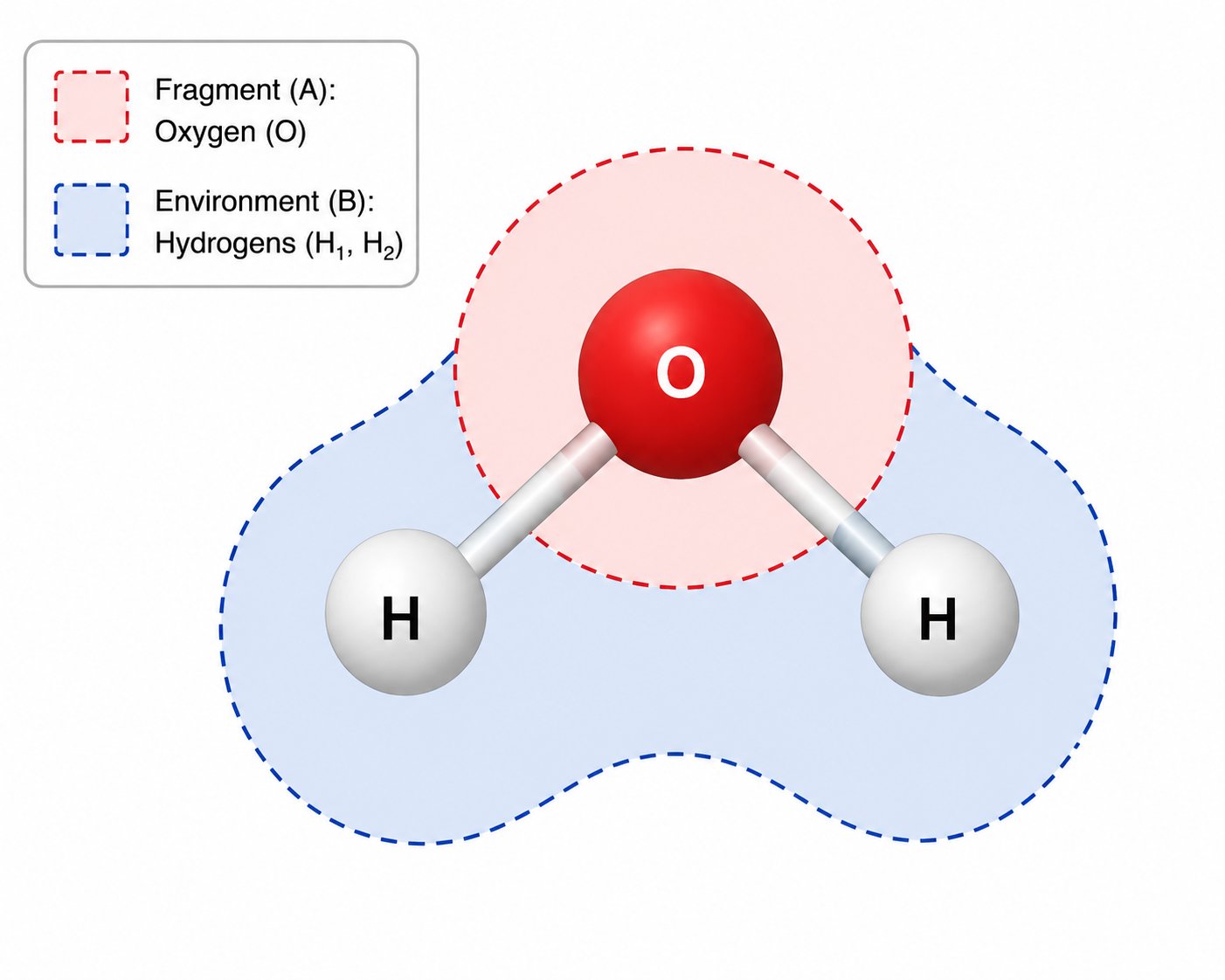

Z_O = 8

Z_H =1

and,

M_O \approx 29157 \text{a.u}

and

M_H\approx 1837 \text{a.u}

Mean-Field Methods

Solving the electronic Schrödinger equation exactly scales exponentially with the number of electrons, so we rely on mean-field methods, in which each electron moves in the averaged field created by all the others. Two common methods underpin the embedding scheme:

Hartree–Fock (HF): approximates the many-electron wavefunction as a single Slater determinant and solves the resulting one-electron (Fock) eigenvalue problem self-consistently. It treats exchange exactly but neglects electron correlation beyond the mean field.

The computational cost is dominated by the two-electron integrals and scales as

O(N_b^4)

, where

N_b

is the number of basis functions.

Density functional theory (DFT): recasts the problem in terms of the electron density $n(\mathbf{r})$ through the Kohn–Sham equations, folding the quantum many-body effects into an approximate exchange–correlation functional (here, B3LYP).

Pure (local/GGA) functionals scale as

O(N_b^3)

. Hybrid functionals such as B3LYP include a fraction of exact exchange, raising the cost to

O(N_b^4)

. Both are solved by a self-consistent field (SCF) iteration and yield the molecular orbitals and density that seed the embedding stage. This tutorial runs the full-system mean field on the Classiq backend using DFT. The detailed HF and DFT formulations are collected in the Technical Notes at the end.

Studied example: mean-field with the Classiq SDK

We now run the full-system mean field for the water molecule. With the SDK we describe the molecule with a MoleculeSpec, create an EmbeddingCalculator, and call run_dft. MoleculeSpec — the molecular description (a frozen dataclass). Its attributes are:

atom (str): the geometry, given as an inline PySCF atom string or the textual contents of a .pdb/.xyz file.

Filesystem paths are not accepted — use the MoleculeSpec.from_pdb_file / MoleculeSpec.from_xyz_file constructors to read a file client-side.

basis (str, default "cc-pVDZ"): the PySCF basis-set name.
charge (int, default 0): the net molecular charge.
spin (int, default 0): 2S, the number of unpaired electrons (0 = closed-shell singlet).
unit (str, default "Angstrom"): the length unit of the coordinates in atom.

EmbeddingCalculator — the pipeline driver. Its constructor takes:

spec (MoleculeSpec): the molecule defined above.
spin_mode (SpinMode, default AUTO): RESTRICTED, UNRESTRICTED, or AUTO (resolves to restricted iff spec.spin == 0); the resolved value is exposed on the read-only effective_spin_mode property.
auto_validations (sequence of ValidationCheck, default empty): checks to run automatically at the end of run_dft_embedding. We leave this empty here and run the checks explicitly in a later section.

Its main methods map to the four-step procedure outlined above:

run_dft corresponds step 1 above. It runs the full-system mean-field (DFT) calculation, returning a DFTState.
run_dft_embedding corresponds to step 2. It partitions the system, builds the embedding potential, and constructs $H_{\text{emb}}$ , returning (MeanFieldData, QuantumData).
Steps 3–4 (solving $H_{\text{emb}}$ with VQE and recovering the total energy) are carried out explicitly in the notebook below.
run_validations: post-hoc consistency diagnostics on the embedding.

The Kohn–Sham (DFT) SCF runs on the backend, and the returned DFTState is a light handle (resolved spin mode, functional, method), while the heavy converged SCF object stays server-side and is threaded automatically into the embedding stage. The consistency checks are run later, in their own section.

!pip install -qq "classiq[chemistry]"

import warnings

import numpy as np
from openfermion.ops import FermionOperator

from classiq.applications.chemistry.embedding import (
    EmbeddingCalculator,
    EmbeddingConfig,
    MoleculeSpec,
    SpinMode,
    ValidationCheck,
)

HARTREE_TO_EV = 27.2114079527

# Water in a standard near-equilibrium geometry (Angstrom).

Atom index 0 is the
# oxygen; indices 1 and 2 are the hydrogens.
spec = MoleculeSpec(
    atom=(
        "O  0.000000   0.000000   0.000000\n"
        "H  0.000000  -0.757000   0.587000\n"
        "H  0.000000   0.757000   0.587000"
    ),
    basis="cc-pVDZ",  # try "sto-3g" for a coarser, faster run
    charge=0,
    spin=0,  # 2S = N_alpha 

- N_beta; 0 => closed-shell singlet
)

calc = EmbeddingCalculator(
    spec,
    spin_mode=SpinMode.AUTO,  # restricted iff spin == 0
)

dft_state = calc.run_dft(xc_functional="B3LYP")
print(f"spin mode : {dft_state.spin_mode}")
print(f"functional: {dft_state.xc_functional}")
print(f"method    : {dft_state.method}")

Output:

spin mode : restricted
  functional: B3LYP
  method    : dft
  

Construction of the Embedding Hamiltonian

After performing the mean field calculation, we partition the total Hilbert space into an active (or alternatively “fragment”) space and the environment space. Following, we derive the embedding Hamiltonian,

H_{\text{emb}}

, which is an effective Hamiltonian of the active space, incorporating averaged environmental effects. Such a calculation is known as a WF-in-MF scheme, i.e., wave-function in a mean-field description. In the present tutorial, MF stands for HF or DFT, and the WF part is conducted by a VQE quantum calculation. There are a number of possible methods by which such an embedding Hamiltonian can be derived. In the present tutorial, we focus on the “Projection (Huzinaga) based embedding”. The key benefit of projection embedding compared to other embedding approaches is that it preserves additivity of the kinetic energy between the fragment (active space) and its environment. As a result, when both subsystems are treated at the same theoretical level, the fragment and environment energies combine to exactly reproduce the total energy of the full system. Within this framework, the total energy is given by:

E_{\text{WF-in-MF}}[{\Psi}_A, \mathbf{D}_A, \mathbf{D}_B] = E_{\text{WF}}[\tilde{\Psi}_A] + E_{\text{MF}}[\mathbf{D}_A + \mathbf{D}_B] - E_{\text{MF}}[\mathbf{D}_A] + \text{tr}\!\left[(\tilde{\mathbf{D}}_{A}-\mathbf{D}_A)\,\mathbf{v}_{\text{emb}}[\mathbf{D}_A, \mathbf{D}_B]\right] + \mu \,\text{tr}[\tilde{\mathbf{D}}_{A}\mathbf{P}_B]~~. \tag{1}

Where

{\Psi}_A

is the wave-function for subsystem

A

. For a classical wave-function method

\tilde{\mathbf{D}}_{A}

is the single-electron reduced density matrix, associated with the state ,

{\Psi}_A

. However, for the quantum calculation such as VQE, one does not generally have efficient access to the density matrix, but to the probablities in the computational basis. Therefore, in the following calculation,

\tilde{\mathbf{D}}_{A}

is obtained by an optimization procedure over the Fock operator of the embedded system (see details below) [2].

E_{\text{WF}}[\tilde{\Psi}_A]

is evaluated by a correlated wave-function calculation, such as VQE. The embedding potential is

\mathbf{v}_{\text{emb}}[\mathbf{D}_A, \mathbf{D}_B] = \mathbf{g}[\mathbf{D}_A +\mathbf{D}_B] - \mathbf{g}[\mathbf{D}_A]~~,

where

\mathbf{g}

includes all the two-electron interactions.

\mu\gg 1

is a model hyperparameter, introducing an energy penalty on the environment states, and

\mathbf{P}_B

is the projection on the environment’s Hilbert space. The construction proceeds in three steps, all carried out automatically by run_dft_embedding (the full derivation of each is collected in the Technical Notes):

Partition the occupied orbitals into the active fragment $A$ and the environment $B$ .

The occupied orbitals are localized and assigned to

A

when their Mulliken weight on the fragment atoms exceeds w_cut, yielding the fragment and environment density matrices

\mathbf{D}_A,\mathbf{D}_B

Build the embedded one-electron Hamiltonian $\mathbf{h}^{A\text{-in-}B} = \mathbf{h} + \mathbf{v}_{\text{emb}}[\mathbf{D}_A,\mathbf{D}_B] + \mu\mathbf{P}_B$ , where $\mathbf{v}_{\text{emb}}$ is the embedding potential, $\mathbf{P}_B = \mathbf{S}\mathbf{D}_B\mathbf{S}$ projects onto the environment, and the level shift $\mu$ keeps the environment orbitals out of the active space.
Select the active space and second-quantize. The fragment-occupied orbitals are augmented with a small set of active virtuals chosen by concentric localization (n_active_virtuals / sv_tol), and the Hamiltonian is expressed in this basis as the embedded second-quantized Hamiltonian $H_{\text{emb}} = \sum_{pq} h_{pq}\,c_p^\dagger c_q + \tfrac{1}{2}\sum V_{pqlm}\,c_p^\dagger c_q^\dagger c_m c_l$ .

Studied example: building the embedding Hamiltonian with the SDK

The entire embedding construction — fragmentation of the occupied space, concentric localization of the active virtuals, assembly of the embedded one-electron operator

h^{A\text{-in-}B}

, and projection to the second-quantized Hamiltonian — is performed in a single run_dft_embedding call. We choose the oxygen atom (index 0) as the active fragment. EmbeddingConfig exposes the following knob: w_cut (Mulliken-weight threshold for assigning orbitals to the fragment), n_active_virtuals (number of concentric-localized virtuals to keep), sv_tol (SVD cutoff used when n_active_virtuals is None), and mu (the level-shift projector strength). The cached DFTState from run_dft is reused automatically.

config = EmbeddingConfig(
    fragment_atoms=(0,),  # oxygen is the active fragment
    xc_functional="B3LYP",
    w_cut=0.3,  # matches the tutorial's oxygen-fragment partition
    n_active_virtuals=3,
    mu=1e6,  # level-shift projector strength
)

mean_field_data, quantum_data = calc.run_dft_embedding(config)

print(f"fragment atom indices      : {mean_field_data.atom_indices}")
print(f"electrons in fragment (A)  : {mean_field_data.n_electrons_A}")
print(f"electrons in environment(B): {mean_field_data.n_electrons_B}")
print(f"fragment DFT energy E_DFT_A : {mean_field_data.E_DFT_fragment:.6f} Ha")

C_active = mean_field_data.C_active
if isinstance(C_active, np.ndarray):
    n_ao, n_mo = C_active.shape
    print(f"active-space MO basis shape: ({n_ao} AOs, {n_mo} MOs)  [restricted]")
else:
    print(
        f"active-space MO basis shapes: "
        f"alpha ({C_active[0].shape[0]} AOs, {C_active[0].shape[1]} MOs), "
        f"beta ({C_active[1].shape[0]} AOs, {C_active[1].shape[1]} MOs)  [unrestricted]"
    )

Output:

fragment atom indices      : (0,)
  electrons in fragment (A)  : 10
  electrons in environment(B): 0
  fragment DFT energy E_DFT_A : -76.420378 Ha
  active-space MO basis shape: (24 AOs, 8 MOs)  [restricted]
  

With

w_{\text{cut}} = 0.3

and the oxygen atom as the fragment, all five occupied molecular orbitals have a Mulliken weight on oxygen that exceeds the threshold. Consequently, all 10 electrons are assigned to subsystem

A

and none to the environment

B

. The active space then consists of these 5 occupied MOs together with the 3 concentric-localized virtual MOs, giving the 8 active-space orbitals reported above.

Consistency Tests

The ValidationCheck diagnostics run through run_validations on the embedding state produced above. We request the DFT-in-DFT energy match, two geometric sanity checks (trace conservation and probability leakage), and the FCI-in-active-space reference in a single call; the results are cached on calc.validation_results. (Alternatively, the cheaper checks can be registered as auto_validations when constructing the EmbeddingCalculator, in which case they run automatically at the end of run_dft_embedding.)

validation_results = calc.run_validations(
    [
        ValidationCheck.DFT_IN_DFT,
        ValidationCheck.TRACE_CONSERVATION,
        ValidationCheck.PROBABILITY_LEAK,
        ValidationCheck.FCI_ACTIVE_SPACE,
    ]
)

for check, (passed, info) in calc.validation_results.items():
    status = "PASS" if passed else "FAIL"
    print(f"{check.value:<22} {status}")
    for key, value in info.items():
        print(f"    {key}: {value}")

Output:

dft_in_dft             PASS
      E_embedded: -76.42037833355558
      E_full: -76.42037833355553
      error: 4.263256414560601e-14
      trace_term: 4.656821072922328e-22
      leakage: 0.0
      dE_mu: 0.0
  trace_conservation     PASS
      trA: 10.000000000000007
      trB: 0.0
      expected: 10
      tol: 1e-08
  probability_leak       PASS
      leak: 0.0
      tol: 1e-08
  fci_active_space       PASS
      E_fci_embedded: -76.03806086432257
      norb_active: 8
      n_particles: [5, 5]
  

Interpreting the validation results: The basic validation results are the dft_in_dft and trace_conservation, verifying physical consistency, while the rest of the validity checks are designed for more advanced usage.

dft_in_dft: Reconstructs the full-system DFT energy from the embedded fragment and environment contributions.

The embedded energy (

\approx -76.420

Ha) matches the full-system energy to

\sim 10^{-13}

Ha, confirming the projection-based embedding is exact when both subsystems use the same level of theory. The vanishing trace_term, leakage, and dE_mu indicate that no density leaked across the partition boundary.

trace_conservation: Verifies that $\text{tr}(\mathbf{D}_A) + \text{tr}(\mathbf{D}_B) = N$ .

Here

\text{tr}_A = 10

and

\text{tr}_B = 0

, summing to the expected 10 electrons.

probability_leak: Checks that the fragment density matrix has no weight on environment orbitals. A leak of $0.0$ confirms a clean separation.
fci_active_space: Runs an exact (FCI) diagonalization of the embedded Hamiltonian within the 8-orbital active space ( $\approx -76.038$ Ha).

This serves as the classical “gold standard” against which the VQE result is compared below.

Quantum-ready Hamiltonians

The embedded and physical Hamiltonians are returned as openfermion.FermionOperator objects on quantum_data, together with the active-space particle numbers and the environment energy correction:

hamiltonian_emb: the embedded Hamiltonian, optimized over the fragment;
hamiltonian_phys: the physical Hamiltonian (used to evaluate the energy);
n_particles: the active-space (n_alpha, n_beta) electron counts;
env_correction: the environment contribution $E_{\text{DFT}}[\mathbf{D}_A+\mathbf{D}_B] - E_{\text{DFT}}[\mathbf{D}_A]$ added back to recover the total energy.

Both Hamiltonians already include the nuclear-repulsion constant.

fermion_hamiltonian_emb = quantum_data.hamiltonian_emb
fermion_hamiltonian_phys = quantum_data.hamiltonian_phys
n_particles = quantum_data.n_particles

print(f"n_particles (alpha, beta)        : {n_particles}")
print(f"# fermionic terms (embedded)     : {len(fermion_hamiltonian_emb.terms)}")
print(f"# fermionic terms (physical)     : {len(fermion_hamiltonian_phys.terms)}")
print(f"environment energy correction    : {quantum_data.env_correction:.6f} Ha")

Output:

n_particles (alpha, beta)        : (5, 5)
  # fermionic terms (embedded)     : 16513
  # fermionic terms (physical)     : 16513
  environment energy correction    : -0.000000 Ha
  

Theory

The Variational Quantum Eigensolver (VQE) is a hybrid algorithm that utilizes a quantum computer to prepare and measure quantum states while a classical computer optimizes them. It is primarily used to find the ground-state energy of a quantum system. The algorithm performs this task as follows (in the following, we omit the subscript

A

for conciseness):

Determine an ansatz state by choosing a parameterized quantum circuit $|{\Psi}(\theta)\rangle = U(\theta)| 0\rangle$ . A good ansatz must be expressive enough to represent the true ground state, while shallow enough to run on the contemporary noisy hardware.
Prepare the quantum state $|\Psi (\theta)\rangle$
Measure the expectation value $E(\theta) = \langle \Psi (\theta)| H_{\text{emb}} | \Psi \rangle$ .
Classical optimization is performed, updating the parameters $\theta$ to reduce the energy.
Repeats until convergence, the resulting state approximates the ground state (by the variational principle) $E(\theta)\geq E_{\text{g.s}} = \min_{\Psi} \langle \Psi | H_{\text{emb}}|\Psi \rangle$

The original variational quantum eigensolver algorithm employed the Unitary Coupled Cluster (UCC) ansatz

| \Psi_{\text{UCC}}\rangle = e^{T-T^\dagger}| 0\rangle~~,

where

T

is the excitation cluster operator that accounts for the correlation eﬀects between the electrons.

T = T_1 + T_2 +\cdots~~,

where

T_k = \frac{1}{(k!)^2}\sum_{ij\dots=1}^{N_\text{occ}}\sum_{ab\dots=1}^{N_\text{vir}}\theta_{ij}^{ab}\tau_{ij}^{ab}

, is the

k

-order excitation operator, with

\tau_{ij}^{ab} = a_{b}^\dagger a_a^\dagger\dots a_j a_i

. This ansatz is a quantum variation of the classical coupled cluster method. In this tutorial, we truncate the cluster operator at first order, retaining only the single excitation operators. This defines the UCCS (Singles) ansatz

| \Psi_{\text{UCCS}}\rangle = e^{T_1- T_1^\dagger}|0\rangle~~,

which yields shallower circuits at the cost of neglecting double excitations. Another option is the hardware-efficient ansatz, which parameterizes the native gates supported by the hardware, e.g., single-qubit rotations and entangling gates for a desired depth. This method enables shallow circuit implementations, but lacks a chemical motivation and may be prone to barren plateaus, which limit the optimization procedure.

Mapping the embedded Hamiltonian to appropriate OpenFermion data structures

We employ the OpenFermion Python library to perform the VQE algorithm with Classiq. OpenFermion is an open-source Python library for working with fermionic systems on quantum computers.

from classiq import *
from classiq.applications.chemistry.hartree_fock import get_hf_state
from classiq.applications.chemistry.mapping import FermionToQubitMapper
from classiq.applications.chemistry.op_utils import qubit_op_to_qmod
from classiq.applications.chemistry.problems import FermionHamiltonianProblem
from classiq.applications.chemistry.ucc import get_ucc_hamiltonians
from classiq.applications.chemistry.z2_symmetries import Z2SymTaperMapper
from classiq.execution.functions import observe
from classiq.execution.functions.minimize import variational_minimize

We inspect the first few terms of the embedded fermionic Hamiltonian:

# Print the first few terms of the embedded Hamiltonian, sorted by operator index
for term, coeff in sorted(fermion_hamiltonian_emb.terms.items(), key=lambda x: x[0])[
    :5
]:
    print(FermionOperator(term, coeff))

Output:

9.188258417746113 []
  -8.514917580385305 [0^ 0]
  0.4377252680041523 [0^ 0^ 0 0]
  -0.0577305403512616 [0^ 0^ 0 1]
  0.005176469296566565 [0^ 0^ 0 2]
  

Studied example: constructing the initial ansatz

We wrap the embedded Hamiltonian in a FermionHamiltonianProblem, taking the active-space particle numbers directly from quantum_data.n_particles, and map it to qubits.

problem = FermionHamiltonianProblem(
    fermion_hamiltonian=fermion_hamiltonian_emb,
    n_particles=n_particles,
)

mapper = FermionToQubitMapper()
num_qubits = mapper.get_num_qubits(problem)
print(f"number of qubits: {num_qubits}")

Output:

number of qubits: 16

We can reduce the problem’s size by identifying

Z2

-symmetries of the embedded Hamiltonian [8]. The reduction is performed by utilizing the Classiq package Z2SymTaperMapper. The transformation reduces the number of qubits from

16

14

. Moreover, the transformation modifies the form of the Hartree-Fock state.

mapper = Z2SymTaperMapper.from_problem(problem)
qubit_ham = mapper.map(problem.fermion_hamiltonian)
# Tapered Hartree-Fock state
hf_state = get_hf_state(problem, mapper)
num_qubits = mapper.get_num_qubits(problem)
print(f"number of qubits after tapering: {num_qubits}")

Output:

number of qubits after tapering: 14

print(f"Encoding of the initial Hartree-Fock state: {hf_state}")

Output:

Encoding of the initial Hartree-Fock state: [True, True, True, True, False, False, False, True, True, True, True, False, False, False]
  

Possibly Trimming the Hamiltonian

The computational resources can be reduced by trimming the qubit Hamiltonian. This corresponds to neglecting Pauli terms whose coefficient in the Hamiltonian is below a certain threshold. Below we trim terms with coefficients below THRESHOLD = 0.1. This is a relatively aggressive threshold that trades accuracy for reduced circuit depth. To preserve more accuracy, decrease the threshold (e.g., 0.01) or comment out the trimming block entirely.

## Trimming the Hamiltonian
THRESHOLD = 0.1
qubit_ham.compress(THRESHOLD)
print(f"Length of trimmed Hamiltonian: {len(qubit_ham.terms)}")

# Defining the SparsePauliOp hamiltonian
HAMILTONIAN = qubit_op_to_qmod(qubit_ham)

Output:


Length of trimmed Hamiltonian: 160

Exact Diagonalization

The exact diagonalization of the trimmed qubit Hamiltonian provides a classical reference for the VQE result. Note that this step scales exponentially with the number of qubits and takes approximately 30 minutes for the 14-qubit problem. The precomputed result is used below to avoid rerunning the expensive calculation.

# Exact diagonalization (uncomment to recompute — takes ~30 min for 14 qubits):
# Hamiltonian_matrix = hamiltonian_to_matrix(HAMILTONIAN)
# eigvals, eigvecs = np.linalg.eig(Hamiltonian_matrix)
# ground_state_energy = np.real(np.min(eigvals))
# print(f"ground state energy: {ground_state_energy}")

ground_state_energy = -77.07666711404943

Solution of the active fragment by VQE

uccsd_hamiltonians = get_ucc_hamiltonians(problem, mapper, excitations=[1])
num_params = len(uccsd_hamiltonians)


@qfunc
def main(params: CArray[CReal, num_params], state: Output[QArray]):
    prepare_basis_state(hf_state, state)
    multi_suzuki_trotter(uccsd_hamiltonians, params, 1, 1, state)


qprog = synthesize(main)

vqe_result = variational_minimize(
    qprog,
    cost_function=HAMILTONIAN,
    initial_params={"params": [0.0] * num_params},
    max_iteration=100,
    tolerance=1e-4,
)

opt_energy, opt_params_dict = vqe_result[-1]
opt_params = np.array(opt_params_dict["params"])

Output:


Submitting job to simulator

Summary of VQE result

print(f"optimized params: {opt_params}")
print(f"optimized energy: {opt_energy}")
print(f"error: {np.abs(100*(opt_energy - ground_state_energy)/ground_state_energy)}%")

Output:

optimized params: [-0.02373629 -0.04936612 -0.05173874 -0.12818058  0.00972557 -0.07164823
   -0.02888005 -0.00773019 -0.01142646  0.00177649 -0.01025428 -0.00280544
   -0.02932838 -0.00967372 -0.03254592 -0.00492063  0.02903898  0.00501263
   -0.01290379 -0.00576706 -0.01757737  0.00317835 -0.00495551 -0.01813467
    0.00355787 -0.03284931  0.06389685 -0.04651961 -0.03327415 -0.01868666]
  optimized energy: -77.31914162597833
  error: 0.31458873483737637%
  

The VQE obtains a ground-state energy within ~1.5% of the exact diagonalization result for the embedded Hamiltonian, confirming the accuracy of the variational approach. Note that the FCI energy from the fci_active_space validation check above provides an equivalent classical reference and can be used in place of the exact diagonalization for benchmarking.

WF-in-DFT Energy Calculation

After obtaining an approximation for the ground state of the embedded Hamiltonian, utilizing the VQE algorithm, we evaluate the energy with respect to the physical Hamiltonian. We introduce an energy_evaluation function which receives a set of parameters and Hamiltonian and evaluates the expectation value with respect to the Hamiltonian. In order to evaluate

E_{WF}[\tilde{\Psi}_A]

(see Eq. (1)) we input the optimized parameters and qubit representation of the physical Hamiltonian, opt_params and qubit_ham_phys.

def energy_evaluation(params, hamiltonian):
    return np.real(observe(qprog, hamiltonian, parameters={"params": params.tolist()}))

problem_phys = FermionHamiltonianProblem(
    fermion_hamiltonian=fermion_hamiltonian_phys,
    n_particles=n_particles,
)

# Reuse the same tapering mapper as the embedded problem.
qubit_ham_phys = mapper.map(problem_phys.fermion_hamiltonian)
qubit_ham_phys.compress(THRESHOLD)
print(f"Length of trimmed physical Hamiltonian: {len(qubit_ham_phys.terms)}")

HAMILTONIAN_PHYS = qubit_op_to_qmod(qubit_ham_phys)

Output:


Length of trimmed physical Hamiltonian: 160

E_WF = energy_evaluation(opt_params, HAMILTONIAN_PHYS)
print(f"E_WF = {E_WF}")

Output:

Submitting job to simulator
  /Users/roiedann/projects/classiq-library/.venv/lib/python3.11/site-packages/classiq/execution/functions/expectation_value.py:167: ClassiqDeprecationWarning: submit_estimate() is deprecated and will no longer be supported starting on 2026-06-22; use submit_observe() instead.
    job = session.submit_estimate(hamiltonian=observable, parameters=parameters)
  Job: https://platform.classiq.io/jobs/752e5b83-e57a-4a9f-a74b-77eb2a193efd
  

Output:


E_WF = -76.94325339004854

Finally, we recover the total WF-in-DFT energy. The physical Hamiltonian already includes the nuclear-repulsion constant, and quantum_data.env_correction supplies the environment term

E_{\text{DFT}}[\mathbf{D}_A+\mathbf{D}_B] - E_{\text{DFT}}[\mathbf{D}_A]

, so the manual recombination of trace and level-shift terms from the original notebook collapses to a single addition:

E_total = E_WF + quantum_data.env_correction
print(f"WF-in-DFT total energy: {E_total} Ha")

Output:


WF-in-DFT total energy: -76.94325339004857 Ha

E_DFT_full = calc.validation_results[ValidationCheck.DFT_IN_DFT][1]["E_full"]
print(f"WF-in-DFT total energy : {E_total:.6f} Ha")
print(f"Full-system DFT energy : {E_DFT_full:.6f} Ha")
print(
    f"Difference (WF 

- DFT)  : {E_total 

- E_DFT_full:.6f} Ha ({(E_total 

- E_DFT_full) * HARTREE_TO_EV:.4f} eV)"
)

Output:

WF-in-DFT total energy : -76.943253 Ha
  Full-system DFT energy : -76.420378 Ha
  Difference (WF 

- DFT)  : -0.522875 Ha (-14.2282 eV)
  

We compare the WF-in-DFT total energy to the full-system DFT energy. Here, the WF-in-DFT energy is a bit lower (more negative) than the pure DFT result by approximately

0.5

Ha (

\sim 14

eV). It is important to note that unlike Hartree–Fock, DFT is not a variational method, and the approximate exchange–correlation functional can introduce systematic biases, particularly in the description of core electrons. Comparing absolute total energies between DFT and correlated methods can therefore be misleading, and a more robust assessment is to examine energy gaps (e.g., excitation energies or reaction energies), where much of the core-electron bias cancels.

Summary

This tutorial demonstrated the full projection-based embedding workflow for a water molecule:

Mean-field calculation: A DFT (B3LYP) SCF was run on the full system via run_dft, yielding converged Kohn-Sham orbitals.
Embedding construction: run_dft_embedding partitioned the occupied space into fragment and environment, built the embedding potential, and produced the second-quantized embedded Hamiltonian.
Validation: Four consistency checks (DFT-in-DFT energy match, trace conservation, probability leak, FCI reference) confirmed the embedding is exact and internally consistent.
VQE optimization: A UCCS (singles) ansatz was optimized on the embedded Hamiltonian, and the result was evaluated against the physical Hamiltonian to recover the total WF-in-DFT energy.

Technical Notes

Hartree-Fock

The Hartree–Fock method provides an approximate, yet tractable, mean-field solution by representing the many-electron wavefunction as a single Slater determinant. The wave-function is approximated as a product of individual electron wave functions, known as the Hartree product:

\psi_{\text{elec}}(\mathbf{x}_1,\dots,\mathbf{x}_N)\approx\phi_1(\mathbf{x}_1)\phi_2(\mathbf{x}_2) \dots \phi_1(\mathbf{x}_N)~~.

Since electrons are indistinguishable particles, we must incorporate the particle statistics by anti-symmetrizing the product form. The anti-symmetrization procedure is conveniently expressed in terms of the so-called Slater determinant

\begin{align} \psi_{\text{elec}}(\mathbf{x}_1, \mathbf{x}_2, \ldots, \mathbf{r}_N) &\approx \frac{1}{\sqrt{N!}} \begin{vmatrix} \phi_1(\mathbf{x}_1) & \phi_2(\mathbf{x}_1) & \cdots & \phi_N(\mathbf{x}_1) \\ \phi_1(\mathbf{x}_2) & \phi_2(\mathbf{x}_2) & \cdots & \phi_N(\mathbf{x}_2) \\ \vdots & \vdots & \ddots & \vdots \\ \phi_1(\mathbf{x}_N) & \phi_2(\mathbf{x}_N) & \cdots & \phi_N(\mathbf{x}_N) \end{vmatrix}~~, \end{align}

where

\phi_j(\mathbf{x_i})

is the value of the

j

‘th spin–orbital evaluated at electron

i

‘th coordinates, and the prefactor

\frac{1}{\sqrt{N!}}

ensures normalization. Each spin-orbital is a product of spatial and spin wave-functions

\phi_j(\mathbf{x}_i)=\phi_j(\mathbf{r}_i,s_i) = \psi_j(\mathbf{r}_i)\chi(s_i)~~.

The calculation of the system’s ground state energy and wavefunction is obtained by employing the variational principle:

The best approximation of the ground state wave-function minimizes the energy

E_{\text{elec}} = \frac{\langle \psi_{\text{elec}}|H_{\text{elec}}| \psi_{\text{elec}}\rangle}{\langle \psi_{\text{elec}}| \psi_{\text{elec}}\rangle } ~~.

By varying the orbitals

\phi_j(\mathbf{x}_i)

under the constraint that they remain orthonormal leads to the Hartree–Fock equations. 2. The variation yields an eigen-like equation for the electron orbital

\{\phi_i\}

F(\mathbf{x}_i) \phi_i (\mathbf{x}_i) = \epsilon_i \phi_i (\mathbf{x}_i)~~.

Here

F(\mathbf{x}_i)= \sum_i h(\mathbf{x}_i) + \sum_{j=1}^{N_{\text{occ}}}\left[J_j(\mathbf{x}_i)- K_j(\mathbf{x}_i)\right]~~,

is effective one-electron operator, called the Fock operator.

$J_j$ is the Coulomb operator (classical electron–electron repulsion)
$K_j$ is the exchange operator (arises from antisymmetry).

The solution of the eigen equation yields the (molecular) electron orbitals

\phi_i

and orbital energies. Because the Fock operator depends on all the orbitals (through the Coulomb and exchange terms), this is a non-linear eigenvalue equation which requires an iterative solution.

A set of basis functions is next defined and the molecular orbitals are expanded as a linear combination of basis functions $\{\chi_\mu\}$ :

\phi_i(\mathbf{x}) = \sum_{\mu} C_{\mu i}\chi_\mu(\mathbf{x})~~,

leading to an equivalent matrix form, known as the Roothan-Hall equation

\mathbf{F}\mathbf{C} = \mathbf{S}\mathbf{C}\mathbf{\epsilon}~~,

where

\mathbf{F}_{\mu\nu} = \langle \chi_\mu |F|\chi_\nu \rangle

and

\mathbf\{S \}_\{\mu\nu\} = \langle \chi_\mu|\chi_\nu \rangle

are the element of the the Fock and Overlap matrices,

\mathbf\{C\}_\{i \mu\} = C_\{\mu i\}

is the coefficient matrix and

\mathbf\{\epsilon\}

is a diagonal matrix containing the orbital energies. The Roothaan-Hall is a generalized eigenfunction equation, which can be solved via classical numerical methods.

Density functional theory

Density functional theory provides a major computational simplification of the electronic problem. The key insight is that the electron density,

n(\mathbf{r}) = 2 \sum_{i=1}^{N_{\text{occ}}}\phi_i^*(\mathbf{r})\phi_i(\mathbf{r}) ~~,

which is a function of only three coordinates, contains a lot of information that is actually observable from the full wave function, which is a function of

3N

coordinates. The theory is based on two fundamental theorems, proved by Kohn and Hohenberg:

The ground-state energy of the Schrodinger equation is a unique functional of the electron density, $E = E[n(\mathbf{r})]$ .
The electron density that minimizes the energy of the overall functional is the true electron density, corresponding to the solution of the Schrodinger equation.

These theorems indicate that the true electron density of the interacting many-body system can be evaluated by finding the density that minimizes the energy functional. The energy functional includes two major contributions:

E[\{ \phi_i \}] = E_{\text{known}}[\{ \phi_i \}] + E_{\text{XC}}[\{ \phi_i \}]~~,

where the first part includes the known contributions: the electronic kinetic energy, and the nuclei-electron, electron-electron, and nuclei-nuclei interactions. The second term, called the exchange-correlation term, includes all the quantum mechanical effects not included in the known term. The task of finding the ground state electron density involves solving the Kohn-Sham equations, each one includes only a single electron:

F^{(\text{KS})}(\mathbf{r})\phi_i^{(\text{KS})}(\mathbf{r}) = \epsilon_i \phi_i^{(\text{KS})}(\mathbf{r})~~,

where the Kohn-Sham operator is given by

F^{(\text{KS})}(\mathbf{r})= \frac{1}{2}\nabla^2 + V_{\text{eN}}(\mathbf{r}) +V_H(\mathbf{r})+V_{XC}(\mathbf{r})~~.

The first two terms represent the kinetic energy and the repulsion potential between the single electron and all the nuclei. The third term, called the Hartree potential, represents the repulsion between the electron and the total electron density

V_H = \int \frac{n(\mathbf{r'})}{|\mathbf{r}-\mathbf{r}'|}d\mathbf{r}' ~~,

created by all electrons, while the last term defines the exchange and correlation contributions to the single-electron equations. It can be defined in terms of a functional derivative of the exchange-correlation contribution

V_{\text{XC}} = \frac{\delta E_{\text{XC}}}{\delta n(\mathbf{r})} ~~.

Note: The Kohn–Sham orbitals are only auxiliary mathematical objects whose only strict physical meaning is to reproduce the exact electron density of the real, interacting system. Similar to the Hartree-Fock equations, due to the dependence of

V_{H}

and

V_{\text{XC}}

, the Kohn-Sham equations are non-linear, and therefore solved iteratively.

We define an initial, trail electron density $n(\mathbf{r})$ .
Solve the Kohn-Sham equations to find the single-particle wave-function $\phi_i^{(\text{KS})}(\mathbf{r})$ , termed the Kohn-Sham wave-functions.
Calculate the electron density $n_{\text{KS}}(\mathbf{r}) = 2 \sum_i\phi_i^{(\text{KS})*}(\mathbf{r})\phi_i^{(\text{KS})}(\mathbf{r})$ .
Check the convergence. If the density converged, stop. Otherwise, update the electron density and return to step
The major caveat of the theory is that the true form of the energy functional $E_{\text{XC}}[\{\phi_i\}]$ is not known and must be approximated. Luckily, for a uniform electron gas, the functional can be derived analytically, providing an initial approximation for the exchange-correlation potential. By evaluating $V_{\text{XC}}$ for a uniform electron gas at the local density, we obtain the so-called local-density approximation (LDA). Alternatively, numerous higher-order approximations offer potentially better results.

Projection-based embedding: detailed derivation

The sections below give the full theory behind the three-step construction summarized in Construction of the Embedding Hamiltonian: partitioning the occupied space into fragment and environment, the projector-based embedding potential, and building the active-space embedded Hamiltonian (including concentric localization of the virtual orbitals). The expression for the embedded system energy,

E_{\text{WF-in-MF}}

, can be understood as an extension of the DFT-in-DFT scheme. In this framework, one writes the total system energy as

E_{\text{DFT-in-DFT}}[\mathbf{D}_{\text{emb},A}, D_B] = E_{\text{DFT}}[\tilde{\mathbf{D}}_{A} + D_B] + \mu \text{tr}[\tilde{\mathbf{D}}_{A} \mathbf{P}_B]

. Minimization of the total energy with respect to system’s

A

density matrix,

{\mathbf{D}}_{\text{emb},A}

, leads to the expression of the Fock matrix of the embedded system,

\mathbf{F}_A

. Self-consistent optimization of

\mathbf{F}_A[\tilde{\mathbf{D}}_{A}] = \mathbf{h}^{\text{A-in-B}}[\mathbf{D}_A,\mathbf{D}_B]+\mathbf{g}[\tilde{\mathbf{D}}_{A}]~~,

with respect to

\tilde{\mathbf{D}}_{A}

, recovers subsystem’s

A

original density matrix

\mathbf{D}_A

. In this sense, the embedding method is internally consistent. The expression for

\mathbf{F}_A

involves a costly re-evaluation of the embedding potential in each SCF iteration. Therefore, to bypass the expensive calculation, one expands the embedding potential to first-order, giving

E_{\text{DFT}}[\tilde{\mathbf{D}}_{A} + \mathbf{D}_B] \approx E_{\text{DFT}}[\tilde{\mathbf{D}}_{A}] + E_{\text{DFT}}[\mathbf{D}_A + \mathbf{D}_B] - E_{\text{DFT}}[\mathbf{D}_A] + \text{tr}[(\tilde{\mathbf{D}}_{A} - \mathbf{D}_A)\mathbf{v}_{\text{emb}}[\mathbf{D}_A, \mathbf{D}_B]]~~.

Here the embedding potential is

\mathbf{v}_{\text{emb}}[\mathbf{D}_A, \mathbf{D}_B] = \mathbf{g}[\mathbf{D}_A + \mathbf{D}_B] - \mathbf{g}[\mathbf{D}_A]

, where

\mathbf{g}

collects all the two-electron mean-field interactions (

\mathbf{J} - \mathbf{K}

for HF,

\mathbf{J} + \mathbf{V}_{\text{XC}}

for DFT). The expression for the total energy of the WF-in-DFT can be understood as a generalization of the DFT-in-DFT method, where the DFT calculation over system

A

is replaced by a correlated wavefunction approach. We divide the WF-in-DFT calculation into three main steps:

Fragmentation of the full system into an active fragment and environment, resulting in localized (or unlocalized) molecular orbitals of the two subsystems.
The MOs of the first mean-field calculation are then used to evaluate the mean-field embedding potential, $\mathbf{v}_{\text{emb}}$ , and the associated embedded Fock operator $\mathbf{F}_A[\tilde{\mathbf{D}}_A]$ .

Solution of the associated Hartree-Fock problem yields optimized MOs that are used for the correlated calculation of system

A

. We denote the optimized MO basis of system

A

\{\tilde{\phi}_i(\mathbf{x})\}

Evaluate the embedded Hamltonian $H_{\text{emb}}$ in the optimized MOs basis.

Each of these steps is detailed in the sections that follow.

Partition of the occupied orbitals into sub-system A (active fragment) and sub-system B (environment)

Before deriving the embedded Hamiltonian, we first must partition the system’s occupied molecular orbitals to the fragment and environment orbitals. Two possible methods are explored: (1) Fragmentation by localized molecular orbitals, and (2) by atomic orbitals.

Fragmentation by localized orbitals

The occupied molecular orbitals

\{\phi_i\}

are delocalized over the entire molecule because they diagonalize the Fock matrix. But chemically, we know the electrons tend to localize: e.g., each bond or lone pair “belongs” roughly to one region of space. To obtain orbitals that reflect this intuition, we rotate the occupied orbitals among themselves using a unitary transformation that spatially localizes each orbital. Formally, we define a unitary

\mathbf{U}

that defines new orbitals:

\mathbf{C}^{(\text{loc})} = \mathbf{C}_{\text{occ}}\mathbf{U}

. The localized orbitals (LOs) span the same occupied subspace (the transformation is unitary), but are much more spatially confined. The Boys and Pipek-Mezey localizations correspond to two different optimization procedures leading to an associated

\mathbf{U}

. Once one has the localized orbitals, we can define the fragment orbitals as the subset of LOs that are mostly on a given set of atoms. Each LO can be projected onto atoms of the fragment using the Mulliken population on the chosen AO subset

w_i = \sum_{\mu\in A} \sum_\nu C^{(\text{loc})\dagger}_{i\mu}S_{\mu \nu} C^{(\text{loc})}_{\nu i}~~,

which indicates the fraction of the

i

‘th MO density on the fragment atoms. Next, we select all localized orbitals for which the population is above a certain threshold,

w_i \geq w_{\text{cut}}

, those

i

‘s correspond to the fragment indices. These indicies allow defining the fragment

A

, and environment

B

, of occupied orbitals

\mathbf{C}_{A} = \mathbf{C}^{(\text{loc})}[:,\text{frag indices}]

\mathbf{C}_{B} = \mathbf{C}^{(\text{loc})}[:,\text{env indices}]

, respectively. Finally, the associated density matrices are evaluated

\mathbf{D}_A =\mathbf{C}_{A}\mathbf{C}_{A}^\dagger ~~~~,~~~~ \mathbf{D}_B =\mathbf{C}_{B}\mathbf{C}_{B}^\dagger ~~.

Note that the localization is performed only on the occupied MO’s, localization of virtual (unoccupied) is unstable and may lead to contradictions within the embedding method.

Fragmentation by atomic orbital

In this fragmentation procedure, we first partition the atomic orbitals into fragment and environment orbitals. Following, we evaluate the Mulliken populations,

\{w_i\}

, of the molecular orbitals. If

w_i

is above a predetermined threshold,

w_{\text{cut}}

, the molecular orbital is included within the fragment Hilbert space. Otherwise, it is set as a part of the environment’s Hilbert space. Similarly, to the fragmentation by localized orbital, the partition of molecular orbitals into two sets, defines

\mathbf{C}_{A}

\mathbf{C}_{B}

, and the associated density matrices

\mathbf{D}_{A}

\mathbf{D}_{B}

Projector-based embedding (PBE) via orthogonal complement

The projector-based embedding introduces a projection operator, allowing the construction of the fragment’s embedded Hamiltonian,

H_{\text{emb}}

. This Hamiltonian governs the dynamics of the fragment system, embedded within the environment. The embedded Hamiltonian includes three main physical contributions:

Kinetic and electron nuclei interaction term, included within the one-electron Hamiltonian term and projected onto the fragment’s Hilbert space.
An embedding potential $\mathbf{v}_{\text{emb}}[\mathbf{D}_A,\mathbf{D}_B]$ which represents the effective interaction between the fragment and environment electrons, projected onto the fragment’s Hilbert space.
The Coulomb repulsion between the fragment electrons.

Following the mean-field calculation on the full system and a partition of the total system into a fragment and environment sub-systems, the evaluation of

H_{\text{emb}}

can be encapsulated in terms of the following steps:

Construct the projection operator, $\mathbf{P}_B = \mathbf{S} \mathbf{D}_B \mathbf{S}$ , where $\mathbf{S}$ is the overlap matrix of the full system.
Evaluate $\mathbf{v}_{\text{emb}}[\mathbf{D}_A, \mathbf{D}_B]$ , the form of which depends on the chosen mean field method.

For a HF calculation (WF-in-HF scheme)

\mathbf{g} = \mathbf{J}-\mathbf{K}

, therefore

\mathbf{v}_{\text{emb}}^{(\text{HF})}[\mathbf{D}_A, \mathbf{D}_B] = \mathbf{J}[\mathbf{D}_A +\mathbf{D}_B] - \mathbf{J}[\mathbf{D}_A] - \mathbf{K}[\mathbf{D}_A +\mathbf{D}_B] + \mathbf{K}[\mathbf{D}_A]~~.

When the mean-field method is chosen to be density functional theory (WF-in-DFT scheme)

\mathbf{g} = \mathbf{J}+\mathbf{V}_{\text{XC}}

, hence,

\mathbf{v}_{\text{emb}}^{(\text{DFT})}[\mathbf{D}_A, \mathbf{D}_B] = \mathbf{J}[\mathbf{D}_A +\mathbf{D}_B] - \mathbf{J}[\mathbf{D}_A] + \mathbf{V}_{\text{XC}}[\mathbf{D}_A +\mathbf{D}_B] - \mathbf{V}_{\text{XC}}[\mathbf{D}_A]~~.

A third possiblity is a hybrid approach, where a combined HF and DFT is utilized for the mean-field calculation, in that case the embedded Hamiltonian would include both exchange and exchange-correlation terms. 4. Gather the terms to construct the one-core Hamiltonian in the AO basis

\{\chi_\mu\}

\mathbf{h}^{\text{A-in-B}} = \mathbf{h} + \mathbf{v}_{\text{emb}}[\mathbf{D}_A, \mathbf{D}_B] + \mu \mathbf{P}_B~~,

where

\mathbf{h}

is the one-electron core Hamiltonian matrix, including the kinetic energy and the electron nuclei interaction terms.

Construct the embedding Hamiltonian

The embedding Hamiltonian is constructed in terms of the system’s

A

MOs, we denote these by

\{\xi_p\}

Occupied (possibly localized) molecular orbitals
Concentric localized virtual orbitals

The fragment-occupied MOs of

\{\xi_p\}

are obtained in the fragmentation procedure of the total system’s occupied. However, virtual orbitals are more spatially extended than occupied ones, moreover, localizing them destroys their energetic and physical ordering, and breaks the clean separation between the active (embedded) space and the environment, making the resulting embedded Hamiltonian ill-conditioned and harder to converge. The truncation of of the number of virtual orbitals and association of a restricted number of virtual orbitals in the fragment’s Hilbert space is achieved by concentric localization.

Concentric localization of virtual orbitals

The partition of virtual orbitals into active fragment and environment virtual orbitals is achieved through concentric localization, which includes only orbitals that have a large overlap (in a pre-defined sense) with the occupied orbitals of the active fragment. Specifically, we employ a one-shell concentric localization procedure, where one selects the active virtual orbitals as the smallest set of virtual MOs that couple most strongly (via the Fock/overlap metric) to the fragment’s occupied localized orbitals, i.e., the first “shell” of virtuals surrounding the fragment. The calculation includes the following steps:

We first obtain a set of canonical virtual orbitals, which contain all the unoccupied MO orbitals.

The orbitals are stored as columns of the matrix C_virt_A, which contains the associated coefficients of the AO basis set.

Compute the coupling matrix $M = C_{\text{virt}}^TSF C_{\text{occ},A}$ , where the columns of $C_{\text{occ,A}}$ correspond to the active fragment’s occupied MOs, and the columns of $C_{\text{virt}}$ correspond to the canonical virtual orbitals $| v_i^{\text{virt}} \rangle$ .

The form of the coupling matrix,

M

, can be understood as follows: The Fock operator

F

constitutes an effective Hamiltonian of the mean-field problem, through which the occupied and virtual orbitals “feel” each other. Applying

F

to an occupied MO answers the question: where can this occupied orbital “go” when excited? Since the AO are not orthogonal, the projector from AO to MO requires an AO overlap correction. Therefore,

SFC_{\text{occ},A}

is a properly normalized way of expressing the operation of the Fock operator on each fragment-occupied orbital and expressing the result in the AO space. Finally, we project the result on the space of virtual orbitals

Perform a singular value decomposition (SVD) of M:

M = U \Sigma V^T~~,

here the columns of

U

are orthonormal combinations of virtual orbitals, ordered by coupling strength (the singular values). 4. We keep the first

k

columns (largest singular values), where

k

is determined by introducing a lower bound threshold, sv_tol, for the singular values. These columns define the active virtual orbitals

C_{\text{virt},A} = C_{\text{virt}}U_{[:,0:k]}~~.

Each column

j

C_{\text{virt},A}

contains the AO coefficients of a linear combination of canonical virtual orbitals with the largest coupling to the occupied space of subsystem

A

, these are the “virtual-concentric localized” orbitals:

| v_{j}^{(CL)}\rangle =\sum_i^{n_{\text{virt }}}| v_i^{\text{virt}} \rangle U_{ij}~~.

Combine the fragment’s occupied MOs and the concentric localized virtual MOs:

C_A = [C_{\text{occ},A}|C_{\text{virt},A}]~~.

Next, we build the embedded Hamiltonian

H_{\text{emb}} = \sum_{p,q=1}^{N_{\text{frag}}} h_{pq} c_{p}^{\dagger} c_{q} + \frac{1}{2}\sum V_{pqlm} c^{\dagger}_{p}c^{\dagger}_{q}c_{m}c_{l}~~,

where

c^\dagger/c

are the second quantization fermionic creation/annihilation operators.

h_{pq} = \langle {\xi}_p |\mathbf{h}^{\text{A-in-B}}|\xi_q \rangle

are the elements of

\mathbf{h}^{\text{A-in-B}}

in the optimized MOs of system

A

V_{pqlm}

are the components of the two-electron Coulomb tensor in the

\{\xi_p(\mathbf{x})\}

basis.

Coulomb Two-Electron Integral

In the orbital basis

\{\phi_\mu\}

, the two-electron repulsion integrals (ERIs) are:

(\mu \nu|\lambda \sigma)=\int\int \phi_{\mu}^*(\mathbf{r}_1) \phi_{\nu} (\mathbf{r_1})\frac{1}{|\mathbf{r}_1-\mathbf{r}_2|}\phi_{\lambda}^*(\mathbf{r}_2) \phi_{\sigma}(\mathbf{r}_2)d \mathbf{r}_1 d \mathbf{r}_2

References

[1]: Rossmannek, M., Pavosevic, F., Rubio, A., & Tavernelli, I. (2023). Quantum embedding method for the simulation of strongly correlated systems on quantum computers. The Journal of Physical Chemistry Letters, 14(14), 3491-3497. [2]: Lee, S. J., Welborn, M., Manby, F. R., & Miller III, T. F. (2019). Projection-based wavefunction-in-DFT embedding. Accounts of chemical research, 52(5), 1359-1368. [3]: Manby, F. R., Stella, M., Goodpaster, J. D., & Miller III, T. F. (2012). A simple, exact density-functional-theory embedding scheme. Journal of chemical theory and computation, 8(8), 2564-2568. [4]: Helgaker, T., Jorgensen, P., & Olsen, J. (2013). Molecular electronic-structure theory. John Wiley & Sons. [5]: Argaman, N., & Makov, G. (2000). Density functional theory: An introduction. American Journal of Physics, 68(1), 69-79. [6]: Baer, R. (2009). Electron density functional theory. Lecture notes, Institute of Chemistry, The Fritz Haber Center for Molecular Dynamics. [7]: Tilly, J., Chen, H., Cao, S., Picozzi, D., Setia, K., Li, Y., … & Tennyson, J. (2022). The variational quantum eigensolver: a review of methods and best practices. Physics Reports, 986, 1-128. [8]: Bravyi, S., Gambetta, J. M., Mezzacapo, A., & Temme, K. (2017). Tapering off qubits to simulate fermionic Hamiltonians. arXiv preprint arXiv:1701.08213.

Algorithms

Applications

Tutorials

Projected Based Embedding Tutorial

View on GitHub

Background: Quantum Chemistry

Mean-Field Methods

Studied example: mean-field with the Classiq SDK

Construction of the Embedding Hamiltonian

Studied example: building the embedding Hamiltonian with the SDK

Consistency Tests

Quantum-ready Hamiltonians

Theory

Mapping the embedded Hamiltonian to appropriate OpenFermion data structures

Studied example: constructing the initial ansatz

Possibly Trimming the Hamiltonian

Exact Diagonalization

Solution of the active fragment by VQE

WF-in-DFT Energy Calculation

Summary

Technical Notes

Hartree-Fock

Density functional theory

Projection-based embedding: detailed derivation

Partition of the occupied orbitals into sub-system A (active fragment) and sub-system B (environment)

Fragmentation by localized orbitals

Fragmentation by atomic orbital

Projector-based embedding (PBE) via orthogonal complement

Construct the embedding Hamiltonian

Concentric localization of virtual orbitals

Coulomb Two-Electron Integral

References

View on GitHub

​Background: Quantum Chemistry

​Mean-Field Methods

​Studied example: mean-field with the Classiq SDK

​Construction of the Embedding Hamiltonian

​Studied example: building the embedding Hamiltonian with the SDK

​Consistency Tests

​Quantum-ready Hamiltonians

​Theory

​Mapping the embedded Hamiltonian to appropriate OpenFermion data structures

​Studied example: constructing the initial ansatz

​Possibly Trimming the Hamiltonian

​Exact Diagonalization

​Solution of the active fragment by VQE

​WF-in-DFT Energy Calculation

​Summary

​Technical Notes

​Hartree-Fock

​Density functional theory

​Projection-based embedding: detailed derivation

​Partition of the occupied orbitals into sub-system A (active fragment) and sub-system B (environment)

​Fragmentation by localized orbitals

​Fragmentation by atomic orbital

​Projector-based embedding (PBE) via orthogonal complement

​Construct the embedding Hamiltonian

​Concentric localization of virtual orbitals

​Coulomb Two-Electron Integral

​References

Background: Quantum Chemistry

Mean-Field Methods

Studied example: mean-field with the Classiq SDK

Construction of the Embedding Hamiltonian

Studied example: building the embedding Hamiltonian with the SDK

Consistency Tests

Quantum-ready Hamiltonians

Theory

Mapping the embedded Hamiltonian to appropriate OpenFermion data structures

Studied example: constructing the initial ansatz

Possibly Trimming the Hamiltonian

Exact Diagonalization

Solution of the active fragment by VQE

WF-in-DFT Energy Calculation

Summary

Technical Notes

Hartree-Fock

Density functional theory

Projection-based embedding: detailed derivation

Partition of the occupied orbitals into sub-system A (active fragment) and sub-system B (environment)

Fragmentation by localized orbitals

Fragmentation by atomic orbital

Projector-based embedding (PBE) via orthogonal complement

Construct the embedding Hamiltonian

Concentric localization of virtual orbitals

Coulomb Two-Electron Integral

References