
View on GitHub

Open this notebook in GitHub to run it yourself
In this notebook we present three ways of approximating the inverse function with Chebyshev polynomials in some spectral interval S=[1,1κ][1κ,1],S= \left[-1,\, -\frac{1}{\kappa}\right] \cup \left[\frac{1}{\kappa},\, 1\right], given the polynomial degree:
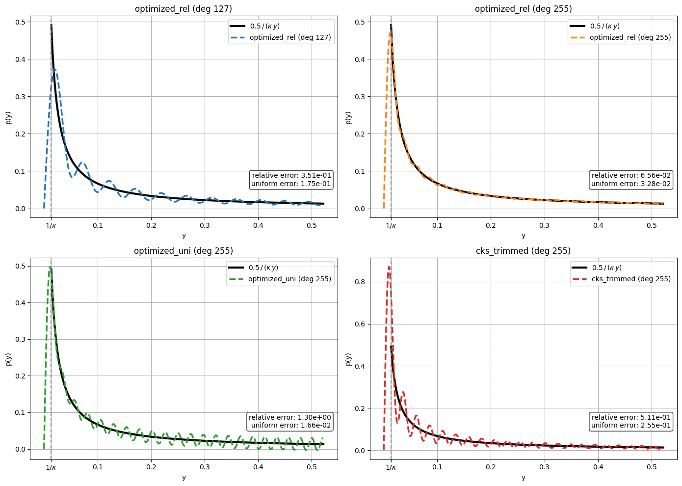
  1. Optimized relative error (optimized_rel): the polynomial p(y)p(y) minimizing
maxySyp(y)1.\max_{y\in S}|y\,p(y)-1|.
  1. Optimized uniform error (optimized_uni): the polynomial p(y)p(y) minimizing
maxySp(y)1/y.\max_{y\in S}|p(y)-1/y|.
  1. CKS trimmed (cks_trimmed): polynomial approximation of the inverse function from the original CKS paper [1], trimmed to the target degree.
The polynomial transformation is given by 1yP(y)=j=0(d1)/2(1)jajT2j+1(y)\Large \frac{1}{y} \approx P(y) = \sum^{(d-1)/2}_{j=0} (-1)^j a_j T_{2j+1}(y) The first two cases are available in Classiq QSP application (see the poly_inversion function). 
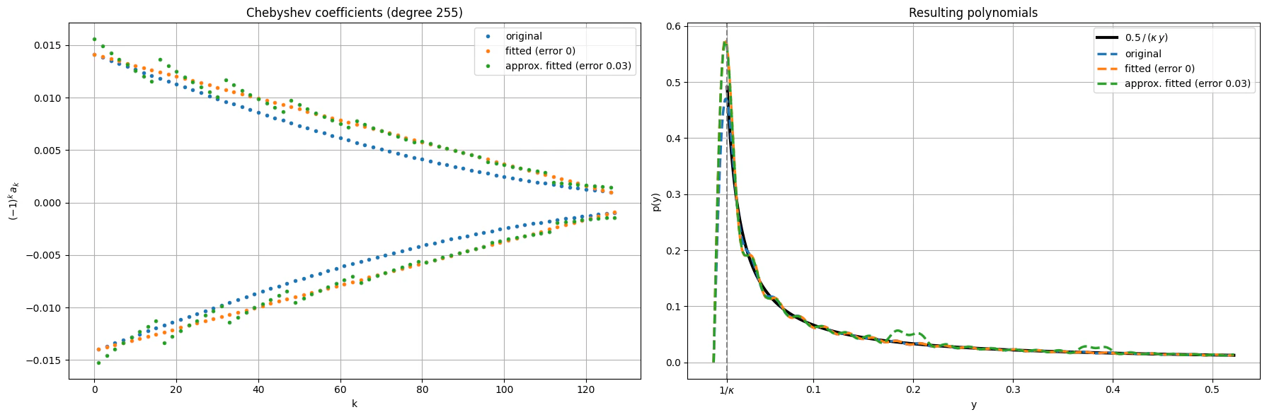
In addition, we consider an approximated transformation, perturbing the polynomial coefficients of those theoretical expansions. This is relevant for reducing gate count in Approximated Chebyshev-LCU quantum linear solvers.
import matplotlib.pyplot as plt
import numpy as np
from banded_be import *
from cheb_utils import fit_linear_coeffs_for_cheb, get_numpy_cheb_trimmed
from numpy.polynomial.chebyshev import Chebyshev
from scipy import sparse
from scipy.special import eval_chebyt

from classiq.applications.chemistry.op_utils import qubit_op_to_qmod
from classiq.applications.qsp.qsp import poly_inversion

import pathlib

path = (
    pathlib.Path(__file__).parent.resolve()
    if "__file__" in locals()
    else pathlib.Path(".")
)

def eval_odd_cheb_poly(coef, x):
    # sum_k coef[k] * T_{2k+1}(x)
    return sum(coef[k] * eval_chebyt(2 * k + 1, x) for k in range(len(coef)))


def compute_approx_errors(coeffs, norm, scale, w_min, w_max, n_points=2000):
    """Return (relative_error, uniform_error) of the polynomial over [w_min, w_max].

Relative error: max |y * p(y) / (scale * w_min) - 1|
    Uniform error:  max |p(y) - scale * w_min / y|
    """
    x = np.linspace(w_min, w_max, n_points)
    p = (scale * w_min / norm) * eval_odd_cheb_poly(coeffs[1::2], x)
    ref = scale * w_min / x
    rel_err = float(np.max(np.abs(x * p / (scale * w_min) - 1)))
    uni_err = float(np.max(np.abs(p - ref)))
    return rel_err, uni_err


ALLOWED_CHEB_APPROX = ["optimized_rel", "optimized_uni", "cks_trimmed"]


def get_cheb_coeff(w_min, degree, scale=1, method="optimized_rel", epsilon=1e-4):
    assert (
        method in ALLOWED_CHEB_APPROX
    ), f"method must be one of {ALLOWED_CHEB_APPROX}, got {method!r}"

    kappa = 1 / w_min
    B = int(kappa**2 * np.log(kappa / epsilon))
    j0 = int(np.sqrt(B * np.log(4 * B / epsilon)))
    theoretical_degree = 2 * j0 + 1
    print(
        f"kappa={kappa:.2f}, theoretical degree for epsilon={epsilon}: {theoretical_degree}"
    )

    if method == "optimized_rel":
        print(f"  -> optimized relative-error polynomial, degree {degree}")
        c, m = poly_inversion(degree, kappa, "relative")
        return scale * c / m, scale / m

    if method == "optimized_uni":
        print(f"  -> optimized uniform-error polynomial, degree {degree}")
        c, m = poly_inversion(degree, kappa, "uniform")
        return scale * c / m, scale / m

    if method == "cks_trimmed":
        print(
            f"  -> CKS degree-{theoretical_degree} polynomial trimmed to degree {degree}"
        )
        return (
            get_numpy_cheb_trimmed(w_min, B, scale, degree, theoretical_degree),
            scale * w_min,
        )

Chebyshev polynomials expansions for different types of error bound definitions

We upload some matrix, and consider its block-encoding. We need the block-encoding scaling factor in order to calculate the effective spectral range of singular-values.
mat_name = "nozzle_008_mat"
matfile = "matrices/" + mat_name + ".npz"
mat_raw_scr = sparse.load_npz(path / matfile)
data_size, block_size, be_scaling_factor, be_qfunc = get_banded_diags_be(mat_raw_scr)

mat_raw = mat_raw_scr.toarray()

svd = np.linalg.svd(mat_raw / be_scaling_factor)[1]
w_min = min(svd)
w_max = max(svd)
scale = 0.5

print(f"min singular value: {w_min:.4f}, max singular value: {w_max:.4f}")

params = [
    {"degree": 127, "method": "optimized_rel"},
    {"degree": 255, "method": "optimized_rel"},
    {"degree": 255, "method": "optimized_uni"},
    {"degree": 255, "method": "cks_trimmed"},
]
Output:
min singular value: 0.0133, max singular value: 0.5218
  

kappa = 1 / w_min
x_vals = np.linspace(0, w_max, 500)
mask = (np.abs(x_vals) >= w_min) & (np.abs(x_vals) <= w_max)

fig, axes = plt.subplots(2, 2, figsize=(14, 10))
axes_flat = axes.flatten()
colors = plt.rcParams["axes.prop_cycle"].by_key()["color"]

for i, p in enumerate(params):
    ax = axes_flat[i]
    coeffs, norm = get_cheb_coeff(w_min, p["degree"], scale=scale, method=p["method"])
    odd_coeffs = coeffs[1::2]
    approx = (scale * w_min / norm) * eval_odd_cheb_poly(odd_coeffs, x_vals)

    rel_err, uni_err = compute_approx_errors(coeffs, norm, scale, w_min, w_max)

    ax.plot(
        x_vals[mask],
        scale * w_min / x_vals[mask],
        "-k",
        label=r"$0.5\,/\,(\kappa\, y)$",
        linewidth=3,
    )
    ax.plot(
        x_vals,
        approx,
        "--",
        color=colors[i % len(colors)],
        label=f'{p["method"]} (deg {p["degree"]})',
        linewidth=2.5,
    )
    ax.axvline(x=w_min, color="gray", linestyle="--", linewidth=1.5)

    auto_ticks = [t for t in ax.get_xticks() if 0 < t < w_max and abs(t - w_min) > 1e-6]
    all_ticks = sorted(auto_ticks + [w_min])
    ax.set_xticks(all_ticks)
    ax.set_xticklabels(
        [r"$1/\kappa$" if abs(t - w_min) < 1e-6 else f"{t:.2g}" for t in all_ticks]
    )

    ax.set_xlabel("y")
    ax.set_ylabel("p(y)")
    ax.set_title(f'{p["method"]} (deg {p["degree"]})')
    ax.legend()
    ax.grid(True)
    ax.text(
        0.98,
        0.15,
        f"relative error: {rel_err:.2e}\nuniform error: {uni_err:.2e}",
        transform=ax.transAxes,
        ha="right",
        va="bottom",
        fontsize=10,
        bbox=dict(boxstyle="round,pad=0.3", fc="white", alpha=0.8),
    )

for j in range(len(params), 4):
    axes_flat[j].set_visible(False)

plt.tight_layout()
plt.show()
Output:
kappa=74.93, theoretical degree for epsilon=0.0001: 2575
    -> optimized relative-error polynomial, degree 127
  kappa=74.93, theoretical degree for epsilon=0.0001: 2575
    -> optimized relative-error polynomial, degree 255
  kappa=74.93, theoretical degree for epsilon=0.0001: 2575
    -> optimized uniform-error polynomial, degree 255
  kappa=74.93, theoretical degree for epsilon=0.0001: 2575
    -> CKS degree-2575 polynomial trimmed to degree 255
  

output

Chebyshev polynomials expansions with non-exact coefficients

We obtain the approximated coefficients loaded by approximate state preparation. This block enters as the PREPARE part in the Chebyshev-LCU approach.
degree = 255
sp_error = 0.03

coeffs, norm = get_cheb_coeff(w_min, degree, scale=scale, method="optimized_rel")

fitted_cheb_coeffs = fit_linear_coeffs_for_cheb(coeffs)
odd_coef = fitted_cheb_coeffs

positive_ind = np.arange(len(odd_coef))[0::2]
positive_fitted = odd_coef[0::2]
negative_ind = np.arange(len(odd_coef))[1::2]
negative_fitted = odd_coef[1::2]
# Calculate prep for Chebyshev LCU
lcu_size_inv = len(odd_coef).bit_length() - 1
odd_coeffs_signs = np.sign(odd_coef)
assert np.all(
    odd_coeffs_signs == np.where(np.arange(len(odd_coeffs_signs)) % 2 == 0, 1, -1)
), "Non alternating signs for odd coefficients"
normalization_inv = sum(np.abs(odd_coef))
prepare_probs_inv = (np.abs(odd_coef) / normalization_inv).tolist()

simulated_amps = []
number_of_ry = []
qprogs = []
for index, err in enumerate([0.0, sp_error]):

    @qfunc
    def main(inv_block: Output[QNum[lcu_size_inv]]):
        allocate(inv_block)
        inplace_prepare_state(prepare_probs_inv, err, inv_block)

    qprog = synthesize(
        main,
        preferences=Preferences(
            custom_hardware_settings=CustomHardwareSettings(
                basis_gates=["cx", "ry", "h", "x", "y", "z", "s", "t"]
            )
        ),
    )

    qprogs.append(qprog)
    print(f"for {err}: {qprog.transpiled_circuit.count_ops}")
    number_of_ry.append(qprog.transpiled_circuit.count_ops["ry"])

    df = calculate_state_vector(qprog)
    abs_simulated_amps = np.zeros(2**lcu_size_inv)
    abs_simulated_amps[df["inv_block"]] = df["probability"]
    simulated_amps.append(
        [
            (-1) ** k * abs_simulated_amps[k] * normalization_inv
            for k in range(2**lcu_size_inv)
        ]
    )
Output:
kappa=74.93, theoretical degree for epsilon=0.0001: 2575
    -> optimized relative-error polynomial, degree 255
  linear fit parameters: slope = -0.00010397734302726349, b= 0.014094618961514994
  

Output:

Submitting job to simulator
  

Output:
for 0.0: {'s': 516, 'h': 264, 'z': 258, 'ry': 127, 'cx': 126}
  

Output:

Job: https://platform.classiq.io/jobs/75e75b1b-1bb7-4208-9122-3668882d2d35
  Submitting job to simulator
  

Output:
for 0.03: {'s': 28, 'h': 16, 'z': 14, 'ry': 11, 'cx': 6}
  

Output:

Job: https://platform.classiq.io/jobs/0080ea0f-de41-4ab5-9048-de541aa7ba40
  

assert number_of_ry[1] < number_of_ry[0] / 2
Next, we plot the approximated coefficients and the resulting polynomial. We can see that for rough approximation, which reduces quantum resources for loading the coefficients on a quantum variable, still gives a good fit.
fig, (ax_a, ax_b) = plt.subplots(1, 2, figsize=(18, 6))

# Plot coefficients
ax_a.plot(coeffs[1::2], ".", markersize=6, label="original")
ax_a.plot(simulated_amps[0], ".", markersize=6, label="fitted (error 0)")
ax_a.plot(
    simulated_amps[1], ".", markersize=6, label=f"approx. fitted (error {sp_error})"
)
ax_a.set_xlabel("k")
ax_a.set_ylabel(r"$(-1)^k\,a_k$")
ax_a.set_title(f"Chebyshev coefficients (degree {degree})")
ax_a.legend()
ax_a.grid(True)

# Plot the resulting polynomial
fac = scale * w_min / norm
poly_orig = fac * eval_odd_cheb_poly(coeffs[1::2], x_vals)
poly_fit = fac * eval_odd_cheb_poly(simulated_amps[0], x_vals)
poly_approx = fac * eval_odd_cheb_poly(simulated_amps[1], x_vals)

ax_b.plot(
    x_vals[mask],
    scale * w_min / x_vals[mask],
    "-k",
    label=r"$0.5\,/\,(\kappa\,y)$",
    linewidth=3,
)
ax_b.plot(x_vals, poly_orig, "--", linewidth=2.5, label="original")
ax_b.plot(x_vals, poly_fit, "--", linewidth=2.5, label="fitted (error 0)")
ax_b.plot(
    x_vals, poly_approx, "--", linewidth=2.5, label=f"approx. fitted (error {sp_error})"
)
ax_b.axvline(x=w_min, color="gray", linestyle="--", linewidth=1.5)

auto_ticks = [t for t in ax_b.get_xticks() if 0 < t < w_max and abs(t - w_min) > 1e-6]
all_ticks = sorted(auto_ticks + [w_min])
ax_b.set_xticks(all_ticks)
ax_b.set_xticklabels(
    [r"$1/\kappa$" if abs(t - w_min) < 1e-6 else f"{t:.2g}" for t in all_ticks]
)
ax_b.set_xlabel("y")
ax_b.set_ylabel("p(y)")
ax_b.set_title("Resulting polynomials")
ax_b.legend()
ax_b.grid(True)

plt.tight_layout()
plt.show()
output

References

[1] Andrew M. Childs, Robin Kothari, and Rolando D. Somma. Quantum algorithm for systems of linear equations with exponentially improved dependence on precision. SIAM Journal on Computing, 46:1920, 2017.