View on GitHub

Open this notebook in GitHub to run it yourself
Grover Mixers for QAOA (GM-QAOA) is one of the algorithms applied to constrained optimization problems, where the mixer operator in QAOA is replaced by a parameterized Grover diffuser operator that utilizes an equal superposition of all feasible solutions [1]. In the potential challenges of standard QAOA, the cost operator (which applies phases based on the objective function) and the mixer operator (which explores the state space) are alternately applied. This method sometimes fails to reach the desired solution in constrained problems. GM-QAOA is a variant of the Quantum Approximate Optimization Algorithm (QAOA) and is particularly designed for constrained optimization problems. In the standard QAOA, the variational circuit alternates between the following two types of unitaries:
  1. Phase-separation operator (based on the cost Hamiltonian H^C\hat{H}_C),
  2. Mixer (a unitary to explore the solution space).
For unconstrained problems, a simple mixer (ieiβXi)(\prod_i e^{-i \beta X_i}) is sufficient. GM-QAOA avoids this difficulty by shifting the complexity of mixer design into the state preparation step.

Exercise

Let’s assume that we will solve the following problem using QAOA and GM-QAOA. We impose the following constraint: i=03xi=1\sum_{i=0}^{3} x_i = 1 The objective function is given by: f(x0,x1,x2,x3)=x0+2(x1+x2+x3)3x2+10x3f(x_0,x_1,x_2,x_3) = x_0 + 2(x_1+x_2+x_3) - 3x_2 + 10x_3 Find x0,x1,x2,x3x_0, x_1, x_2, x_3 that minimize ff.

Algorithm description

In GM-QAOA, a Grover-type mixer is introduced: UM(β)=eiβFF,U_M(\beta) = e^{-i \beta |F\rangle\langle F|}, where F|F\rangle is the equal superposition of all feasible solutions: F=1FxFx.|F\rangle = \frac{1}{\sqrt{|F|}} \sum_{x \in F} |x\rangle. If we define U^S\hat{U}_S as the unitary that generates F|F\rangle from the initial state 0n|0\rangle^{\otimes n}, U^S0n=F,\hat{U}_S |0\rangle^{\otimes n} = |F\rangle, then the GM-QAOA circuit of depth pp can be expressed as: β,γ=U^M(βp)U^P(γp)U^M(β1)U^P(γ1)U^S0n,|\beta,\gamma\rangle = \hat{U}_M(\beta_p) \hat{U}_P(\gamma_p) \cdots \hat{U}_M(\beta_1) \hat{U}_P(\gamma_1) \hat{U}_S |0\rangle^{\otimes n}, where U^P(γ)=eiγH^C.\hat{U}_P(\gamma) = e^{-i\gamma \hat{H}_C}.

Approach 1: QAOA

First, lets try to implement general QAOA.
Output:
Output:
Output:
Output:
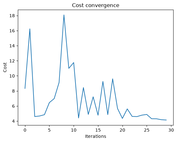
output
Output:

Approach 2: GM-QAOA

Next, we use GM-QAOA.
Output:
Output:
Output:
Output:
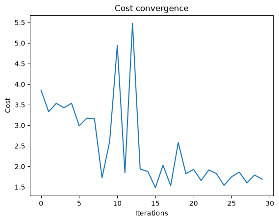
output
Output:
Output:
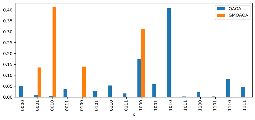
output When x=0010x = 0010, the minimum value becomes f=1f = -1, and GM-QAOA exhibits a stronger amplification effect compared to QAOA.

References

[1]: A. Bärtschi, S. Eidenbenz. “Grover Mixers for QAOA: Shifting Complexity from Mixer Design to State Preparation” arXiv:2006.00354 (2020).