Value at Risk (VaR) is a widely used financial risk metric that estimates the maximum expected loss of a portfolio over a given time horizon at a specified confidence level, based on the probability distribution of returns.Classical VaR calculations for complex portfolios often rely on Monte Carlo simulations, which can be computationally expensive and slow to converge.Quantum computing can improve this process by using Iterative Quantum Amplitude Estimation (IQAE) to estimate loss probabilities more efficiently. IQAE provides a quadratic speedup over classical Monte Carlo methods by estimating expected values with fewer samples, without requiring deep quantum circuits.This makes it particularly suitable for near-term quantum hardware and enables faster, more accurate VaR calculations for high-dimensional and non-linear financial portfolios.
As a first step, we have to model the problem mathematically. We will use a simple yet powerful model, which captures the essence of portfolio optimization:First, we will import the Python libraries required for this implementation. Classiq, of course, and Numpy.
import matplotlib.pyplot as pltimport numpy as npimport scipyfrom classiq import *from classiq.applications.iqae.iqae import IQAE
Now, we will define the parameters required for the Value at Risk process, and create the probability distribution function.
# How many qubits we want the quantum circuit to benum_qubits = 7# Mu (μ) represents the Averagemu = 0.7# Sigma (σ) represents the Standard Deviationsigma = 0.13# The Alpha (α) parameter represents the probability in which P(X > v) = 1 - αALPHA = 0.07# Find Alpha in a given precisionTOLERANCE = ALPHA / 10def get_log_normal_probabilities(mu_normal, sigma_normal, num_points): log_normal_mean = np.exp(mu + sigma**2 / 2) log_normal_variance = (np.exp(sigma**2) - 1) * np.exp(2 * mu + sigma**2) log_normal_stddev = np.sqrt(log_normal_variance) # cutting the distribution 3 sigmas from the mean low = np.maximum(0, log_normal_mean - 3 * log_normal_stddev) high = log_normal_mean + 3 * log_normal_stddev print(log_normal_mean, log_normal_variance, log_normal_stddev, low, high) x = np.linspace(low, high, num_points) return x, scipy.stats.lognorm.pdf(x, s=sigma_normal, scale=np.exp(mu_normal))# %%grid_points, probs = get_log_normal_probabilities(mu, sigma, 2**num_qubits)
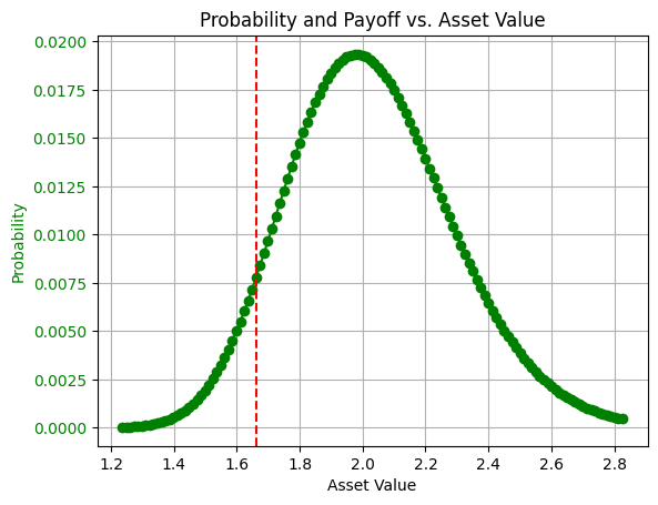
In order to have a benchmark to our solution, and since the problem space is not too big, let’s calculate the Value at Risk classically, and plot the probability distribution function.
probs = (probs / np.sum(probs)).tolist()fig, ax1 = plt.subplots()# Plotting the log-normal probability functionax1.plot(grid_points, probs, "go-", label="Probability") # Green line with circlesax1.tick_params(axis="y", labelcolor="g")ax1.set_xlabel("Asset Value")ax1.set_ylabel("Probability", color="g")# Adding grid and titleax1.grid(True)plt.title("Probability and Payoff vs.Asset Value")VAR = 0# Find the value at risk ALPHA of grid_pointsaccumulated_value = 0for index in range(len(probs)): accumulated_value += probs[index] if accumulated_value > ALPHA: VAR = grid_points[index] breakprint(f"Value at risk at {int(ALPHA*100)}%: {VAR}")# Plot the vertical line of VaR at 5%ax1.axvline(x=VAR, color="r", linestyle="--", label="VaR at 5%")
The Binary Search Approach To Calculate Value At Risk
We can solve the Value at Risk use-case also with a binary search approach.This approach will benefit us from a complexity perspective once we will integrate the quantum function that calculates alpha given an index.
# This function calculates the alpha classically given the index and the list of probabilitiesdef calc_alpha(index: int, probs: list[float]): sum_probs = sum([probs[i] for i in range(index)]) return sum_probs
# This function updates the new index based on the comparison between the measured alpha value and the required value.# The search size correlates with the current binary search step.def update_index(index: int, required_alpha: float, alpha_v: float, search_size: int): if alpha_v < required_alpha: return index + search_size return index - search_size
# This is the main Value at Risk function, which gets the required probability (required_alpha), the index and the alpha calculation function# We aim to use calc_alpha defined abovedef print_status(v, alpha_v, search_size, index): print(f"v: {v}, alpha_v: {alpha_v}") print(f"{search_size=}") print(f"{index=}") print("------------------------")def print_results(grid_points, index, probs): print(f"Value at risk at {ALPHA*100}%: {grid_points[index]})") global VAR print(f"Real VaR", VAR) return indexdef value_at_risk(required_alpha, index, calc_alpha_func=calc_alpha): v = probs[index] alpha_v = calc_alpha_func(index, probs) search_size = index // 2 print_status(v, alpha_v, search_size, index) # Tolerance represents the accuracy of the alpha we aim to get while (not np.isclose(alpha_v, required_alpha, atol=TOLERANCE)) and search_size > 0: index = update_index(index, required_alpha, alpha_v, search_size) # Binary search, divided by 2 - as we know the function is always growing in that part of the graph. search_size = search_size // 2 v = grid_points[index] alpha_v = calc_alpha_func(index, probs) print_status(v, alpha_v, search_size, index) print_results(grid_points, index, probs)
Value at Risk using Iterative Quantum Amplitude Estimation (IQAE)
Iterative Quantum Amplitude Estimation (IQAE) is a key algorithm in the quantum computing toolbox. It is useful for quantum-enhanced Monte Carlo methods, which are in use for several important quantum finance applications like Value at Risk (VaR) estimation.The goal of Quantum Amplitude Estimation (QAE) is to estimate the probability (or amplitude) of a certain outcome from a quantum circuit.Compared to other classical methods, some has been presented above in this notebook - it is potentially quadratically faster.IQAE is a NISQ-friendly version of the traditional Quantum Amplitude Estimation (QAE), and includes the following stages:
State preparation encoding the desired probabilty, in this case - for not losing more than $X for an asset or a portfolio of asset.
Use controlled applications of the Grover operator (unlike QAE, which utilises Fourier Transform)
Measure and update the estimate using classical methods.
Defining The State Preparation for the IQAE Algorithm
In order to use IQAE, we need to define the state preparation function, which includes two main parts:
Loading the distribution of the asset values into a quantum state.
Defining the payoff function, which marks the states where the asset value is below a certain threshold (the index in this case).
For the first part, we will use Classiq’s inpalce_prepare_state function.For the second part, we will define a simple comparison operation using Classiq’s arithmetic library.
written_qmod = Falsedef calc_alpha_quantum(index: int, probs: list[float]): # Global variable global GLOBAL_INDEX GLOBAL_INDEX = index # Creation of the model, given the constratins and the circuit preferences iqae = IQAE( state_prep_op=state_preparation, problem_vars_size=num_qubits, constraints=Constraints(max_width=28), preferences=Preferences(machine_precision=num_qubits), ) qprog = iqae.get_qprog() global written_qmod qmod = iqae.get_model() if not written_qmod: written_qmod = True show(qprog) iqae_res = iqae.run(epsilon=0.05, alpha=0.01) # Result of the iterative QAE # iqae_res = res[0].value measured_payoff = iqae_res.estimation confidence_interval = np.array( [interval for interval in iqae_res.confidence_interval] ) print("Measured Payoff:", measured_payoff) print("Confidence Interval:", confidence_interval) return measured_payoff
index = get_initial_index()
var = value_at_risk(ALPHA, index, calc_alpha_quantum)