Grover's Search Algorithm

View on GitHub

Open this notebook in GitHub to run it yourself

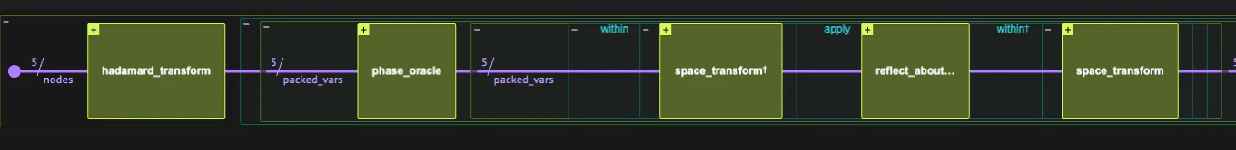
Grover’s Search Algorithm, introduced by Lov Grover in 1996 [1], is one of the canonical quantum algorithms. It provides a quadratic speedup for searching an unstructured database and is often considered alongside Shor’s algorithm as a cornerstone of quantum computing. The search algorithm has applications in various fields, such as in cybersecurity.

Input: A Boolean function (oracle) $f: \{0,1\}^n \rightarrow \{0,1\}$ marking “solutions” among $N = 2^n$ possible items.

Promise: At least one marked element exists in the search space.

Output: With high probability, the algorithm outputs a marked element $x$ (i.e., $f(x) = 1$ ).

Complexity: The algorithm requires $O(\sqrt{N})$ oracle queries to obtain the result, while the query complexity for classical search is $O(N)$ .
Keywords: Search and optimization, Unstructured search, Quadratic speedup, Amplitude amplification, Graph problems, SAT problems, Oracle/Query complexity.

Grover’s Search algorithm starts with preparing the search space

|s\rangle

, and then repeats over a combination of two reflection operations:

U_f|x\rangle = (-1)^{f(x)}|x\rangle \qquad \text{usually called an "Oracle", adds a minus phase to marked states, and}

U_s = 2|s\rangle\langle s|-1 \qquad \text{usually called a "Diffuser", reflects around the full search space.}

The number of times we need to repeat the combination of these two reflections (sometimes called a “Grover Operator”) depends on the number of solutions: for

k

solutions in a search space of size

N

, we shall perform

r\sim \pi \sqrt{N/k}

iterations. In practice, however, the number of solutions is often unknown. In that case, one can perform a quantum counting algorithm prior to the search, or run the search algorithm repeatedly, with an increasing number of repetitions

r_i\sim \frac{\pi}{4} \sqrt{2^i}

for

i=0,1,\dots

. Both approaches do not affect the complexity of the search algorithm. In this notebook we take the second approach. For a given problem, Grover’s algorithm depends on two functions, one for preparing the search space and another for applying the oracle, as well as on the number of repetitions. Below we address two canonical search problems, a 3-SAT problem and a Max-Cut problem on a graph. In this notebook we work with the grover_operator function, and define a classical postprocess function for iterating over different

r

values and obtianing the marked states. Using the phase_oracle quantum function from the Classiq open-library together with the Qmod language for high-level problem definitions helps avoid low-level implementation details that are typically required on other platforms.

Classical postprocess function

Below we define a function that runs a quantum program of the Grover’s search algorithm, for an increasing number of repetitions, until a marked state is found.

import numpy as np

from classiq import *
from classiq.qmod.symbolic import pi


def repeat_grover_until_success(
    grover_search_qprog, classical_formula, num_shots=1000, threshold=0.45, max_iter=4
):
    """
    Runs a grover_search_qprog with different powers, given by a CInt parameter `r`.
    """
    i = 0
    r_previous = None
    with ExecutionSession(
        grover_search_qprog, ExecutionPreferences(num_shots=num_shots)
    ) as es:
        while i < max_iter:
            r = int(np.ceil(np.pi / 4 * np.sqrt(2**i)))
            if r == r_previous:
                # skip duplicate r
                i += 1
                continue

            print(f"running Grover with {r} repetitions")
            res = es.sample({"r": r})

            for sample in res.parsed_counts:
                if (
                    classical_formula(**sample.state)
                    and sample.shots / num_shots > threshold
                ):
                    print(
                        f"Success! a solution was found with probability larger than {threshold}, using {r} repetitions"
                    )
                    return res, r

            r_previous = r
            i += 1
    print(
        f"Could not find a solution, try to in increase max_iter or decrease the threshold, returning last run."
    )
    return res, r

Example: 3-SAT problem

The 3-SAT problem [2] is a famous

\text{NP-Complete}

problem, a solution of which allows solving any problem in the complexity class

\text{NP}

. We treat two different 3-SAT problems, a small one and a larger one. For illustration, we define a function for printing the truth table of SAT problems.

import itertools


def print_truth_table(num_variables, boolean_func):
    variables = [f"x{i}" for i in range(num_variables)]
    combinations = list(itertools.product([0, 1], repeat=num_variables))

    header = "  ".join([f"{var:<5}" for var in variables]) + " | Result"
    print(header)
    print("-" * len(header))

    for combination in combinations:
        result = boolean_func(list(combination)) != 0  # pass as array
        values_str = "  ".join([f"{val:<5}" for val in combination])
        print(f"{values_str} | {result:<5}")

We start with a small problem:

Small 3-SAT formula

We specify a 3-SAT formula in the so-called Conjunctive Normal Form (CNF), that requires a solution:

(x_1 \lor x_2 \lor x_3) \land (\neg x_1 \lor x_2 \lor x_3) \land (\neg x_1 \lor \neg x_2 \lor \neg x_3) \land (\neg x_1 \lor \neg x_2 \lor x_3) \land (x_1 \lor x_2 \lor \neg x_3) \land (\neg x_1 \lor x_2 \lor \neg x_3)

NUM_VARIABLES = 3


def small_3sat_formula(x):
    return (
        (x[0] | x[1] | x[2])
        & (~x[0] | x[1] | x[2])
        & (~x[0] | ~x[1] | ~x[2])
        & (~x[0] | ~x[1] | x[2])
        & (x[0] | x[1] | ~x[2])
        & (~x[0] | x[1] | ~x[2])
    )

We can see that the formula has two possible solutions:

print_truth_table(NUM_VARIABLES, small_3sat_formula)

Output:

x0     x1     x2    | Result
  ----------------------------
    0      0     | 0    
    0      1     | 0    
    1      0     | 1    
    1      1     | 1    
    0      0     | 0    
    0      1     | 0    
    1      0     | 0    
    1      1     | 0
  

We define the Grover search model for finding the solution. To specify the model, we use the standard phase_oracle that transforms ‘digital’ oracle; i.e.,

|x\rangle|0\rangle \rightarrow |x\rangle|f(x)\rangle

to a phase oracle

|x\rangle \rightarrow (-1)^{f(x)}|x\rangle

. The predicate that we pass to the phase oracle is simply given by the 3-CNF formula defined above.

@qperm
def sat_oracle(x: Const[QArray], res: QBit):
    res ^= small_3sat_formula(x)


@qfunc
def main(r: CInt, x: Output[QArray[NUM_VARIABLES]]):
    allocate(x)
    hadamard_transform(x)

    power(
        r,
        lambda: grover_operator(
            lambda vars: phase_oracle(sat_oracle, vars), hadamard_transform, x
        ),
    )


qprog_small_3sat = synthesize(main, constraints=Constraints(max_width=20))


show(qprog_small_3sat)

Output:

Quantum program link: https://platform.classiq.io/circuit/3CIkfrlgj5kqpn5Xs2FvtKKfF5p
  

We execute our repeat until success function:

res_3_sat_small, r = repeat_grover_until_success(qprog_small_3sat, small_3sat_formula)

Output:

running Grover with 1 repetitions
  Success! a solution was found with probability larger than 0.45, using 1 repetitions
  

We can see that a single iteration was needed to find solutions with high probability:

n_solutions = 3
df = res_3_sat_small.dataframe
df_new = df.head(n_solutions).copy()
first_col = df.columns[0]
df_new["f(x)"] = df_new[first_col].apply(small_3sat_formula)
print("The quantum search result:")
df_new

Output:


The quantum search result:

	x	counts	probability	bitstring	f(x)
0	[0, 1, 1]	510	0.51	110	1
1	[0, 1, 0]	490	0.49	010	1

Large 3-SAT formula

We continue with a larger example:

def large_3sat_formula(x):
    return (
        (x[1] | x[2] | x[3])
        & (~x[0] | x[1] | x[2])
        & (~x[0] | x[1] | ~x[2])
        & (~x[0] | ~x[1] | x[2])
        & (x[0] | ~x[1] | ~x[2])
        & (x[0] | ~x[1] | x[2])
        & (~x[0] | ~x[1] | ~x[3])
        & (~x[0] | ~x[1] | x[3])
        & (~x[1] | ~x[2] | ~x[3])
        & (x[1] | ~x[2] | x[3])
        & (x[0] | ~x[2] | x[3])
        & (x[0] | ~x[1] | ~x[3])
        & (~x[0] | ~x[1] | ~x[2])
    )


NUM_VARIABLES_LARGE = 4
print_truth_table(NUM_VARIABLES_LARGE, large_3sat_formula)

Output:

x0     x1     x2     x3    | Result
  -----------------------------------
    0      0      0     | 0    
    0      0      1     | 1    
    0      1      0     | 0    
    0      1      1     | 1    
    1      0      0     | 0    
    1      0      1     | 0    
    1      1      0     | 0    
    1      1      1     | 0    
    0      0      0     | 0    
    0      0      1     | 0    
    0      1      0     | 0    
    0      1      1     | 0    
    1      0      0     | 0    
    1      0      1     | 0    
    1      1      0     | 0    
    1      1      1     | 0
  

The procedure is identical to the small use-case, just changing small_3sat_formula to large_3sat_formula.

@qperm
def sat_oracle(x: Const[QArray], res: QBit):
    res ^= large_3sat_formula(x)


@qfunc
def main(r: CInt, x: Output[QArray[NUM_VARIABLES_LARGE]]):
    allocate(x)
    hadamard_transform(x)

    power(
        r,
        lambda: grover_operator(
            lambda vars: phase_oracle(sat_oracle, vars), hadamard_transform, x
        ),
    )


qprog_large_3sat = synthesize(main, constraints=Constraints(max_width=24))
show(qprog_large_3sat)
res_3_sat_large, r = repeat_grover_until_success(qprog_large_3sat, large_3sat_formula)

Output:

Quantum program link: https://platform.classiq.io/circuit/3CIkkbehGecuMHmQCrZjWQdl8fg
  running Grover with 1 repetitions
  running Grover with 2 repetitions
  Success! a solution was found with probability larger than 0.45, using 2 repetitions
  

We can print the five most probable solutions:

n_solutions = 5
df = res_3_sat_large.dataframe
df_new = df.head(n_solutions).copy()
first_col = df.columns[0]
df_new["f(x)"] = df_new[first_col].apply(large_3sat_formula)
df_new

	x	counts	probability	bitstring	f(x)
0	[0, 0, 1, 1]	475	0.475	1100	1
1	[0, 0, 0, 1]	471	0.471	1000	1
2	[0, 1, 1, 0]	6	0.006	0110	0
3	[0, 1, 1, 1]	6	0.006	1110	0
4	[0, 1, 0, 0]	5	0.005	0010	0

We can see that the amplitude of the two “marked” solutions is amplified.

Example: Graph Cut Search Problem

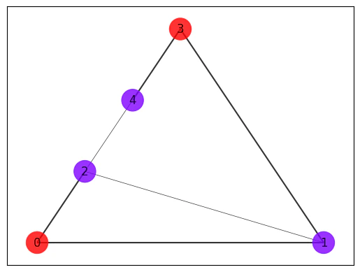
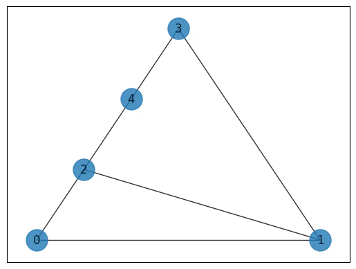
The “Maximum Cut Problem” (MaxCut) [3] is an example of a combinatorial optimization problem. It refers to finding a partition of a graph into two sets, such that the number of edges between the two sets is the maximum. The MaxCut problem is defined as follows: Given a graph

G=(V,E)

with

|V|=n

nodes and

E

edges, a cut is defined as a partition of the graph into two complementary subsets of nodes. The gaol is to find a cut where the number of edges between the two subsets is the maximum. We can represent a cut, and the number of its connecting edges as follows:

$x\in \{0,1\}^n$ is a binary vector of size $n$ that represents a cut: assigning 0 and 1 to nodes in the first and second subsets, respectively.
$C(x)=\sum_{(i,j)}x_i (1-x_j)+x_j (1-x_i)=\sum_{(i,j)}x_i \oplus x_j$ gives the number of connecting edges for a given cut.

The MaxCut problem cannot be cast directly into a Grover’s search algorithm, as we task to find the maximum of a function, rather than some “marked” solutions. One approach is to apply Grover’s algorithms for formulas of the form

C(x)\geq T

, for some fixed value of

T

: We initialize a threshold

T

, then run Grover’s algorithm with an oracle that marks cuts with

C(x)\geq T

to amplify promising candidates. If a better cut is found, we update

T

and repeat until no improvement is likely (or a preset budget is reached). In this notebook we show a solution for a single instance of this procedure, i.e., taking one example with some value for

T

. We initiate a specific graph whose maximum cut is 5:

import networkx as nx

# Create graph
G = nx.Graph()
G.add_nodes_from([0, 1, 2, 3, 4])
G.add_edges_from([(0, 1), (0, 2), (1, 2), (1, 3), (2, 4), (3, 4)])
pos = nx.planar_layout(G)
nx.draw_networkx(G, pos=pos, with_labels=True, alpha=0.8, node_size=500)

Constructing a Grover’s search algorithm is done in similar to the 3-SAT examples, we only require to define a predicate formula. In this example we set the cut size (the value of

T

) to

CUT_SIZE = 4

# cut formulas
def is_cross_cut_edge(x1: int, x2: int) -> int:
    return x1 ^ x2

def cut(x):
    return sum(is_cross_cut_edge(x[node1], x[node2]) for (node1, node2) in G.edges)

def cut_predicate(cut_size, x):
    return cut(x) >= cut_size

@qperm
def cut_oracle(cut_size: CInt, nodes: Const[QArray], res: QBit):
    res ^= cut_predicate(cut_size, nodes)


@qfunc
def main(r: CInt, nodes: Output[QArray[len(G.nodes)]]):
    allocate(nodes)
    hadamard_transform(nodes)

    power(
        r,
        lambda: grover_operator(
            lambda vars: phase_oracle(
                lambda vars, res: cut_oracle(CUT_SIZE, vars, res), vars
            ),
            hadamard_transform,
            nodes,
        ),
    )


qprog_max_cut = synthesize(main, constraints=Constraints(max_width=22))
show(qprog_max_cut)

Output:

Quantum program link: https://platform.classiq.io/circuit/3CIknLQwkWvbPUceQC1xGH0fZWK
  

# In this example we reduce the threshold, since typically, more than one solution is expected
res_max_cut, r = repeat_grover_until_success(
    qprog_max_cut, lambda nodes: cut_predicate(CUT_SIZE, nodes), threshold=0.1
)

Output:

running Grover with 1 repetitions
  Success! a solution was found with probability larger than 0.1, using 1 repetitions
  

Upon printing the result, we see that our execution of Grover’s algorithm successfully found the satisfying assignments for the input formula:

n_solutions = 32
df = res_max_cut.dataframe
df_new = df.head(n_solutions).copy()
first_col = df.columns[0]
df_new["f(x)"] = df_new[first_col].apply(lambda x: cut_predicate(CUT_SIZE, x))
df_new

	nodes	counts	probability	bitstring	f(x)
0	[1, 0, 0, 1, 0]	111	0.111	01001	True
1	[0, 1, 1, 0, 0]	108	0.108	00110	True
2	[1, 0, 0, 0, 1]	108	0.108	10001	True
3	[1, 0, 1, 1, 0]	103	0.103	01101	True
4	[0, 1, 1, 1, 0]	97	0.097	01110	True
5	[0, 1, 0, 0, 1]	94	0.094	10010	True
6	[0, 1, 1, 0, 1]	89	0.089	10110	True
7	[0, 0, 1, 1, 0]	87	0.087	01100	True
8	[1, 1, 0, 0, 1]	85	0.085	10011	True
9	[1, 0, 0, 1, 1]	79	0.079	11001	True
10	[0, 0, 0, 0, 0]	4	0.004	00000	False
11	[0, 0, 1, 1, 1]	4	0.004	11100	False
12	[0, 1, 0, 1, 0]	3	0.003	01010	False
13	[0, 1, 0, 1, 1]	3	0.003	11010	False
14	[1, 0, 1, 1, 1]	3	0.003	11101	False
15	[1, 1, 1, 1, 1]	3	0.003	11111	False
16	[1, 0, 0, 0, 0]	2	0.002	00001	False
17	[1, 0, 1, 0, 0]	2	0.002	00101	False
18	[1, 1, 1, 0, 0]	2	0.002	00111	False
19	[0, 0, 1, 0, 1]	2	0.002	10100	False
20	[1, 1, 1, 0, 1]	2	0.002	10111	False
21	[0, 1, 0, 0, 0]	1	0.001	00010	False
22	[0, 0, 1, 0, 0]	1	0.001	00100	False
23	[1, 1, 0, 1, 0]	1	0.001	01011	False
24	[1, 1, 1, 1, 0]	1	0.001	01111	False
25	[0, 0, 0, 0, 1]	1	0.001	10000	False
26	[1, 0, 1, 0, 1]	1	0.001	10101	False
27	[0, 0, 0, 1, 1]	1	0.001	11000	False
28	[1, 1, 0, 1, 1]	1	0.001	11011	False
29	[0, 1, 1, 1, 1]	1	0.001	11110	False

The satisfying assignments are ~100 times more probable than the unsatisfying assignments. We print the corresponding graph for one of them:

result_parsed = df_new["nodes"][0]

import matplotlib.pyplot as plt

edge_widths = [
    is_cross_cut_edge(
        int(result_parsed[i]),
        int(result_parsed[j]),
    )
    + 0.5
    for i, j in G.edges
]
node_colors = [int(c) for c in result_parsed]
nx.draw_networkx(
    G,
    pos=pos,
    with_labels=True,
    alpha=0.8,
    node_size=500,
    node_color=node_colors,
    width=edge_widths,
    cmap=plt.cm.rainbow,
)

References

[1]: L. K. Grover, “A fast quantum mechanical algorithm for database search”, Proceedings of the 28th Annual ACM Symposium on Theory of Computing (STOC ’96), pp. 212–219, 1996. [2]: The 3-SAT problem [3]: The Maximum Cut problem

Algorithms

Applications

Functions

Tutorials

Grover's Search Algorithm

View on GitHub

Classical postprocess function

Example: 3-SAT problem

Small 3-SAT formula

Large 3-SAT formula

Example: Graph Cut Search Problem

References

Algorithms

Applications

Functions

Tutorials

View on GitHub

​Classical postprocess function

​Example: 3-SAT problem

​

​Small 3-SAT formula

​

​Large 3-SAT formula

​Example: Graph Cut Search Problem

​References

Classical postprocess function

Example: 3-SAT problem

Small 3-SAT formula

Large 3-SAT formula

Example: Graph Cut Search Problem

References