View on GitHub

Open this notebook in GitHub to run it yourself
Adiabatic Quantum Computing (AQC) leverages the adiabatic theorem to solve computational problems by gradually evolving a quantum system from an initial ground state to the ground state of a problem-specific Hamiltonian (see the AQC tutorial). This tutorial focuses on applying the AQC approach to solve the Quantum Linear Systems Problem (QLSP), a cornerstone problem in quantum computing with significant applications in fields like machine learning, physics, and optimization. Specifically, we aim to demonstrate how to utilize AQC to approximate the solution to the QLSP [1]. This problem involves finding a quantum state that corresponds to the solution of a linear system of equations. The tutorial provides a structured overview of the QLSP, its mathematical formulation, and the steps needed to transform it into an eigenvalue problem, laying the foundation for solving it within the AQC framework. *This demonstration follows the [1] paper. This notebook was written in collaboration with Prof. Lin Lin and Dr. Dong An, the authors of the paper.*

Problem Statement

Given a Hermitian positive-definite matrix AA and a vector b|b\rangle, the goal is to approximate x|x\rangle-the solution to the linear system Ax=bA|x\rangle=|b\rangle-as a quantum state. We are given:
  • Matrix ACN×NA \in \mathbb{C}^{N \times N}, an invertible Hermitian and positive-definite matrix with condition number κ\kappa and A2=1\|A\|_2 = 1.
  • Vector bCN|b\rangle \in \mathbb{C}^N, a normalized vector.
  • Target Error ϵ\epsilon, specifying the desired accuracy.
The goal is to prepare a quantum state xa|x_a\rangle, which is an ϵ\epsilon-approximation of the normalized solution x=A1b/A1b2|x\rangle = A^{-1}|b\rangle / \|A^{-1}|b\rangle\|_2. The approximation satisfies xaxaxx2ϵ.\| |x_a\rangle \langle x_a| - |x\rangle \langle x| \|_2 \leq \epsilon.

Transformation into AQC

The QLSP is converted into an equivalent eigenvalue problem to leverage quantum computation. This involves the following steps.

  1. Constructing H0H_0
Define: H0=σxQb=[0QbQb0],H_0 = \sigma_x \otimes Q_b = \begin{bmatrix} 0 & Q_b \\ Q_b & 0 \end{bmatrix}, where Qb=INbbQ_b = I_N - |b\rangle \langle b| is a projection operator orthogonal to b|b\rangle. Key properties:
  • H0H_0 is Hermitian.
  • The null space of H0H_0: Null(H0)=span(b~,bˉ)\text{Null}(H_0) = \text{span}(|\tilde{b}\rangle, |\bar{b}\rangle), where
b~=0,b=[b0],bˉ=1,b=[0b].|\tilde{b}\rangle = |0, b\rangle = \begin{bmatrix} b \\ 0 \end{bmatrix}, \quad |\bar{b}\rangle = |1, b\rangle = \begin{bmatrix} 0 \\ b \end{bmatrix}.
The null space of a matrix AA is the set of all vectors x\mathbf{x} such that Ax=0.A\mathbf{x} = 0. With regards to eigenstates and eigenvalues:
  • The null space corresponds to the eigenspace of AA associated with the eigenvalue 00.
  • Any vector in the null space is an eigenvector of AA with eigenvalue 00.

  1. Constructing H1H_1
Define: H1=σ+(AQb)+σ(QbA)=[0AQbQbA0],H_1 = \sigma_+ \otimes (AQ_b) + \sigma_- \otimes (Q_bA) = \begin{bmatrix} 0 & AQ_b \\ Q_bA & 0 \end{bmatrix}, where σ±=12(σx±iσy)\sigma_\pm = \frac{1}{2}(\sigma_x \pm i\sigma_y). Key properties:
  • If AxbA|x\rangle \propto |b\rangle, then QbAx=Qbb=0Q_bA|x\rangle = Q_b|b\rangle = 0.
  • Null space of H1H_1: Null(H1)=span(x~,bˉ)\text{Null}(H_1) = \text{span}(|\tilde{x}\rangle, |\bar{b}\rangle), where
x~=0,x=[x0],|\tilde{x}\rangle = |0, x\rangle = \begin{bmatrix} x \\ 0 \end{bmatrix}, \quad

  1. Adiabatic Interpolation
Construct an interpolation Hamiltonian: H(f(s))=(1f(s))H0+f(s)H1,0s1,H(f(s)) = (1 - f(s))H_0 + f(s)H_1, \quad 0 \leq s \leq 1, where f(s)f(s) is a monotonic function mapping [0,1][0,1][0, 1] \to [0, 1].

  1. Spectral Gap
  • QbQ_b is a projection operator, and the spectral gap between 00 and the rest of the eigenvalues of H0H_0 is 11.
  • For H1H_1, the gap between 00 and the rest of the eigenvalues is bounded from below by 1/κ1/\kappa. [1]

  1. Adiabatic Evolution and Null Space
Note that there is a degeneracy in the number of null states (unlike the regular adiabatic algorithm usage where we typically look at a single ground state): \text{Null}(H_1) = \text{span}(|\tilde{x}\rangle, |\bar{b}\rangle)$.$ We also note that for any $s$, $|\bar{b}\rangle$ is always in the null space of $H(f(s))$; i.e., |\bar{b}\rangle \in \text{Null}(H(f(s))). Therefore, there exists an additional statestate $|\tilde{x(s)}\rangle = |0\rangle \otimes |x(s)\rangle$, such that \text{Null}(H(f(s))) = {|\tilde{x(s)}\rangle, |\bar{b}\rangle}. In particular: - At $s = 0$, $|\tilde{x(0)}\rangle = |\tilde{b}\rangle$, the initial state. - At $s = 1$, $|\tilde{x(1)}\rangle = |\tilde{x}\rangle$, the solution state. Thus, $|\tilde{x(s)}\rangle$ state represents the desired **adiabatic path** for the evolution [[1](#QLSP)]. ## AQC Approach to Solving QLSP The adiabatic quantum algorithm prepares the zero-energy state $|\tilde{x}\rangle$ of $H_1$ as follows: 1. Initialize in the ground state of $H_0$; i.e., $|\tilde{b}\rangle$. 2. Slowly evolve the system by varying $f(s)$ from $f(0) = 0$ to $f(1) = 1$. 3. At the end of the evolution, the system approximates $|\tilde{x}\rangle$, embedding $|x\rangle$, which is the solution of the QLSP. Goals: - **Set up a QLSP example:** Derive $H_0$, $H_1$ and define the interpolation Hamiltonian. - **Quantum circuit design:** Implement Hamiltonian simulation for $H(f(s))$. - **Evaluate results:** Compare quantum simulation results with the numeric calculation. --- Let's begin with the mathematical setup and continue on to implementation.

Setting up a QLSP Example Where A Is a 4x4 Matrix

For simplicity, we first assume A is Hermitian and positive definite.
As a purely mathematical preprocessing step, we calculate the condition number kk for AA.
In practical scenarios, the condition number is often approximated or known beforehand based on external factors or prior knowledge.
Output:

Constructing H0H_0 and H1H_1

The setup_QLSP function prepares the necessary Hamiltonians and normalized components to solve the Quantum Linear Systems Problem (QLSP). The built-in matrix_to_hamiltonian function, used in the setup_QLSP function, encodes the Hamitonian matrix into a sum of Pauli strings that is used to exponentiate the Hamiltonians with a product formula (Suzuki-Trotter) in the next step.

Defining the Interpolation Hamiltonian

For the sake of simplicity, we first use the “vanilla AQC” linear scheduling function f(s(t))=s(t)=t/Tf(s(t)) = s(t) = t / T to define the time-dependent interpolated Hamiltonian, where T is the total evolution time. As tt progresses from 0 to TT, f(s)f(s) satisfies the [0,1][0,1][0, 1] \to [0, 1] mapping.

Analyzing the Spectral Gap

From the quantum adiabatic theorem [3, Theorem 3] the formula for the adiabatic error bound η\eta at any point ss is η(s)=C{H(1)(0)2TΔ2(0)+H(1)(s)2TΔ2(f(s))+1T0s[H(2)(s)2Δ2(f(s))+H(1)(s)22Δ3(f(s))]ds}.\eta(s) = C \left\{ \frac{\|H^{(1)}(0)\|^2}{T \Delta^2(0)} + \frac{\|H^{(1)}(s)\|^2}{T \Delta^2(f(s))} + \frac{1}{T} \int_0^s \left[ \frac{\|H^{(2)}(s')\|^2}{\Delta^2(f(s'))} + \frac{\|H^{(1)}(s')\|^2}{2\Delta^3(f(s'))} \right] ds' \right\}. See Appendix A for a detailed explanation of the components. The formula shows that the adiabatic error is minimized when
  1. The total runtime TT is large (slow evolution).
  2. The spectral gap Δ\Delta is large (well-separated ground and excited states).
  3. The derivatives H(1)\|H^{(1)}\| and H(2)\|H^{(2)}\| are small (smooth Hamiltonian changes).
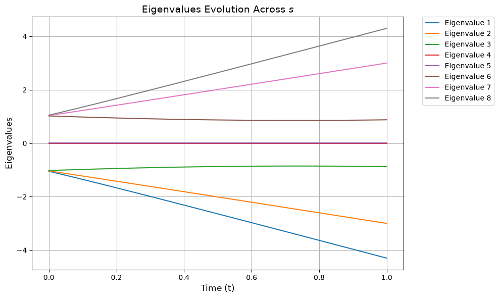
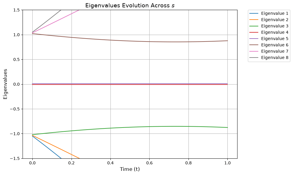
The following function plots the spectral gap Δ\Delta evolution:
output To focus on the spectral gap from the null states, we can zoom in on our plot:
output We can visually observe from the above that although the spectral gap does change throughout ss it still stays quite large in our example, so we can choose TT accordingly. Without going into detail we choose a simple value for TT (represented as TOTAL_EVOLUTION_TIME). However, if we simply assume H(1)2\|H^{(1)}\|^2, H(2)2\|H^{(2)}\|^2 are bounded by constants, and use the worst-case bound that Δκ1\Delta \geq \kappa^{-1}, it can be shown that to have η(1)ϵ\eta(1) \leq \epsilon, the runtime of vanilla AQC is Tκ3/ϵT \propto \kappa^3 / \epsilon.

Implementing AQC

Since ψT(s)=Texp(iT0sH(f(s))ds)ψT(0) ,|\psi_T(s) \rangle = \mathcal{T}\exp \left( -iT \int_0^s H(f(s')) ds' \right) |\psi_T(0) \rangle \ , where T\mathcal{T} is the time-ordering operator, it is sufficient to implement an efficient time-dependent Hamiltonian simulation of H(f(s))H(f(s)). One straightforward approach to achieve this is using the Trotter splitting method. The lowest order approximation takes the form Texp(iT0sH(f(s))ds)m=1Mexp(iThH(f(sm)))\mathcal{T}\exp \left( -iT \int_0^s H(f(s')) ds' \right) \approx \prod_{m=1}^M \exp \left( -iTh H(f(s_m)) \right) which can further be approximated as m=1Mexp(iTh(1f(sm))H0)exp(iThf(sm)H1)\prod_{m=1}^M \exp \left( -iTh(1 - f(s_m)) H_0 \right) \exp \left( -iTh f(s_m) H_1 \right) where h=s/M,sm=mh.h = s/M, s_m = mh. It is proved in [2] that the error of such an approximation is O(poly(log(N))T2/M),\mathcal{O}(\text{poly}(\log(N)) \cdot T^2 / M), which indicates that to achieve an ϵ \epsilon-approximation, it suffices to choose M=O(poly(log(N))T(ϵ)2/ϵ).M = \mathcal{O}(\text{poly}(\log(N)) \cdot T(\epsilon)^2 / \epsilon). (Note that in our case TT also depends on ϵ\epsilon.)

Building the Quantum Model

Using the Classiq platform, we implement the adiabatic path with Suzuki-Trotter decomposition for Hamiltonian exponentiation. In our model TT is represented by the TOTAL_EVOLUTION_TIME and MM is represented by NUM_STEPS. In the Trotter implementation, MM scales as O(T2)O(T^2) with respect to the runtime TT, therefore this is our rough choice of MM:
We are now ready to build our quantum model. The adiabatic_evolution_qfunc function implements the adiabatic path with Suzuki-Trotter decomposition for Hamiltonian exponentiation:
To solve the QLSP we first prepare the H0H_0 zero state b~|\tilde{b}\rangle and then initiate the evolution:

Synthesizing, Verifying, and Executing

Synthesize the model into a quantum program, verify it, and execute it on a state vector simulator:
Output:

Evaluating the Results

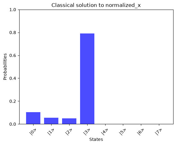
Output:
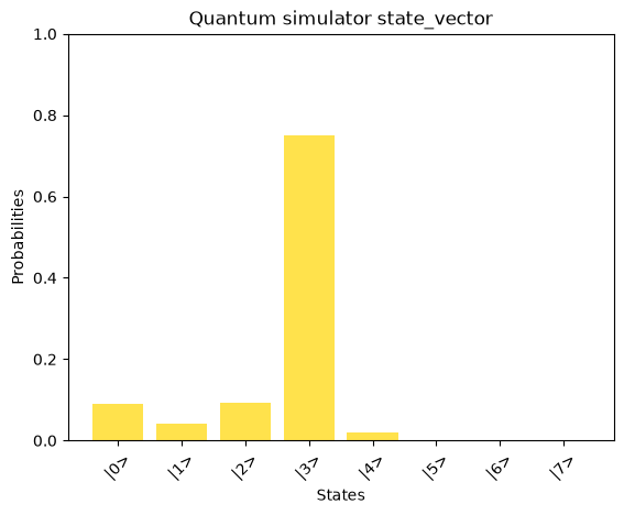
output output
Output:
By comparing the quantum-computed results with the mathematically expected solution, we observe a good alignment, showcasing the potential of the AQC approach for solving linear problems. We can observe the runtime of the above implementation by analyzing the depth parameter from the transpiled circuit data of our quantum program:
Output:
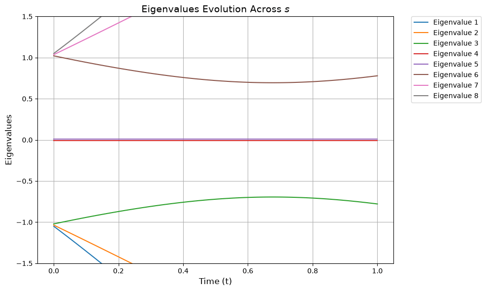
For alternative QLSP configurations, it may be necessary to select different values for TT and MM, and these choices will naturally impact the circuit depth. For instance:
Output:
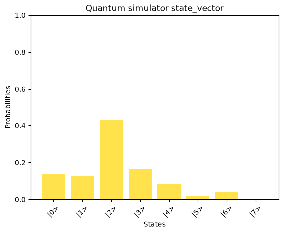
output Although the condition number is higher, the spectral gap remains relatively large. However, using the same values of TT and MM as chosen above result in an increased error:
Output:
Output:
output output
Output:
Output:
Choosing TT and MM accordingly improves results but affects the overall runtime:
Output:
Output:
output output
Output:
Output:
As expected, the overall circuit depth increases to achieve a high degree of similarity in the results. Although the results are satisfying, a more optimal approach can be implemented based on the discrete adiabatic theorem [4].
Important: The implementation example above aims to provide an intuitive understanding of the principles behind solving quantum linear solver problems with the adiabatic quantum evolution and the associated error bounds. However, for simplicity and accessibility, several aspects of the implementation are not optimal:
  • Suzuki-Trotter Decomposition: We utilized the first order Suzuki-Trotter approximation for time evolution. As such (as mentioned above), a more optimal approach based on the discrete adiabatic theorem [4] could be implemented.
  • Schedule Function: We used the vanilla AQC scheduling function. Using more sophisticated scheduling functions as suggested in [1] will improve runtime.
  • Brute-Force Encoding: The encoding of Pauli operators in this tutorial is direct and unoptimized, scaling exponentially with system size. Other encoding techniques (such as suggested in [4]) will be more efficient.
These choices were made to prioritize conceptual clarity over computational efficiency. The next step would be to apply state-of-the-art techniques and show improvement in gate complexity and runtime.

Appendix A: Explanation of the Adiabatic Error-bound Components

The adiabatic error bound η(s)\eta(s) is defined by the quantum adiabatic theorem [3, Theorem 3]: η(s)=C{H(1)(0)2TΔ2(0)+H(1)(s)2TΔ2(f(s))+1T0s[H(2)(s)2Δ2(f(s))+H(1)(s)22Δ3(f(s))]ds}.\eta(s) = C \left\{ \frac{\|H^{(1)}(0)\|^2}{T \Delta^2(0)} + \frac{\|H^{(1)}(s)\|^2}{T \Delta^2(f(s))} + \frac{1}{T} \int_0^s \left[ \frac{\|H^{(2)}(s')\|^2}{\Delta^2(f(s'))} + \frac{\|H^{(1)}(s')\|^2}{2\Delta^3(f(s'))} \right] ds' \right\}. Detailed explanation of components:
  1. η(s)\eta(s):
  • Represents the adiabatic error bound at a specific point s[0,1]s \in [0, 1].
  • Quantifies the deviation of the quantum state from the ground state during evolution.
  1. CC:
  • A proportionality constant that depends on system-specific properties such as the dimensionality and scaling of norms.
  1. H(1)(0)\|H^{(1)}(0)\|:
  • The operator norm of the first derivative of the Hamiltonian, H(s)H(s), evaluated at s=0s = 0.
  • Indicates how quickly the Hamiltonian initially changes.
  1. TT:
  • The total runtime of the adiabatic evolution.
  • Larger TT values reduce the error, as slower evolution aids adiabaticity.
  1. Δ(0)\Delta(0):
  • The spectral gap at s=0s = 0, defined as the energy difference between the ground state and the first excited state of H(s)H(s).
  • Larger gaps improve the adiabatic process.
  1. H(1)(s)\|H^{(1)}(s)\|:
  • The operator norm of the first derivative of H(s)H(s) at an intermediate point ss.
  • Reflects how fast the Hamiltonian changes during evolution.
  1. Δ(f(s))\Delta(f(s)):
  • The spectral gap at the point ss, mapped via the function f(s)f(s).
  1. H(2)(s)\|H^{(2)}(s')\|:
  • The operator norm of the second derivative of the Hamiltonian, H(2)(s)H^{(2)}(s'), at a point ss'.
  • Captures the curvature or acceleration of the Hamiltonian’s evolution.
  1. 0sds\int_0^s \cdots ds':
  • An integral from 00 to ss, summing contributions of the Hamiltonian’s derivatives over the path.
  • Accounts for cumulative effects of the Hamiltonian’s changes during evolution.
  1. Δ2(f(s))\Delta^2(f(s')) and Δ3(f(s))\Delta^3(f(s')):
  • Higher powers of the spectral gap at ss'.
  • Larger gaps (in Δ2\Delta^2 and Δ3\Delta^3) significantly reduce the adiabatic error.

References

[1]: An, D. and Lin, L. 2022. “Quantum Linear System Solver Based on Time-Optimal Adiabatic Quantum Computing and Quantum Approximate Optimization Algorithm.” ACM Trans. Quantum Comput. 3. arXiv:1909.05500 [2]: Wim van Dam, Michele Mosca, and Umesh Vazirani. 2001. How powerful is adiabatic quantum computation? In Proceedings 42nd IEEE Symposium on Foundations of Computer Science. IEEE, Piscataway, NJ, 279–287. [3]: Sabine Jansen, Mary-Beth Ruskai, and Ruedi Seiler. 2007. Bounds for the adiabatic approximation with applications to quantum computation. J. Math. Phys. 48, 10, 102111. [4]: [The discrete adiabatic quantum linear system solver has lower constant factors than the randomized adiabatic solver. Pedro C.S. Costa, Dong An, Ryan Babbush, Dominic Berry](https://arxiv.org/abs/2312.07690).