

View on GitHub
Open this notebook in GitHub to run it yourself
Generative AI, especially through Generative Adversarial Networks (GANs), revolutionizes content creation across domains by producing highly realistic output. Quantum GANs further elevate this potential by leveraging quantum computing, promising unprecedented advancements in complex data simulation and analysis.
In this notebook, we explore the concept of Quantum Generative Adversarial Networks (QGANs) and implement a simple QGAN model using the Classiq SDK. We study a simple use case of a Bars and Stripes dataset. We begin with a classical implementation of a GAN, and then move to a hybrid quantum-classical GAN model.
1 Data Preparation
We generate the Bars and Stripes dataset, a simple binary dataset consisting of 2x2 images with either a horizontal or vertical stripe pattern:1.1 Visualizing the Generated Data
Let’s plot a few samples from the dataset to visualize the bars and stripes patterns: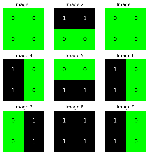
2 Classical Network
2.1 Defining a Classical GAN
We begin by defining the generator and discriminator models (architecture) for the classical GAN. We work withtensorboard to save our logs (uncomment the following line to install the package):
2.2 Training a Classical GAN
We define the training loop for the classical GAN:'generator_model.pth':
Output:
Output:
2.3 Evaluating the Performance
Output:
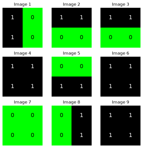
3 Quantum Hybrid Network Implementation
In this section we define a quantum generator circuit and integrate it into a hybrid quantum-classical GAN model. We then train the QGAN model and evaluate its performance.3.1 Defining the Quantum GAN
3.1.1 Defining the Quantum Generator
We define the three components of the quantum layer. This is where the quantum network architect’s creativity comes into play! The design we choose:- Data encoding - we take a
datum_angle_encodingthat encodes data points on qubits. - A variational ansatz - we combine RY and RZZ gates.
- Classical postprocess - we take the vector , with being the probability to measure 1 on the -th qubit.
main quantum function, and synthesize it into a quantum program.
Output:
Output:
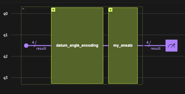
Hierarchical view of the quantum circuit for the QGAN generator.
The circuit consists of an angle encoding layer, an ansatz layer, and a postprocessing layer
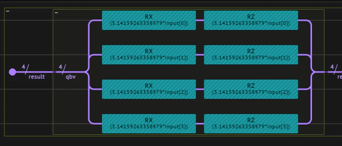
Angle encoding layer consists of two consecutive noncommuting rotations encoding a single datum.
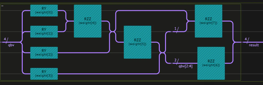
Ansatz layer including parametrized rotation followed by a pair-wise entangler via the RZZ gate sequence.
3.1.2 Defining the Hybrid Network
We define the network building blocks: the generator and discriminator in a hybrid network configuration with a quantum layer,3.3 Training the QGAN
We can use the training loops defined above for the classical GAN:q_logs directory. We also use Tensorboard to monitor the training in real time. It is possible to use an online version - which is more convenient - but for the purpose of this notebook we use the local version. An example of a vizualization output that can be obtained from tensorboard is shown in the next figure.

Example of two training sessions. The first (green) line depicts a process in which the loss function estimator is rising; a clear indication that the learning session does not seem to converge to the desired result. The second (orange) line shows the convergence of both. The two components compete to improve their performance.
Since training can take long time to run, we take a pre-trained model, whose parameters are stored in
q_generator_trained_model.pth. In addition, we take a smaller sample size of
- (The pre-trained model was trained on 1000 samples.) To train a randomly initialized QGAN, change
num_samplesfrom 250 to 1000 for the data creation, andnum_epochsfrom 1 to 10 in the training calltrain_gan.
Output:
3.3 Evaluating the Performance
Finally, we can evaluate the performance of the QGAN, similar to the classical counterpart:Output:
Output:
Why do you think the accuracy is so high? Answer: The system chose a metastable pathway where no violation of the rules occurs! Try longer training, different sets of hyperparameters, different architectures, etc.