Matrix Inversion with Quantum Singular Value Transform (QSVT)

View on GitHub

Open this notebook in GitHub to run it yourself

Quantum Matrix Inversion (or Quantum Linear Solver) via QSVT provides a framework for solving linear systems exponentially faster than known classical methods under certain conditions [1]. The algorithm employs a polynomial transformation of singular values to block-encode the inverse of a matrix, which can then be applied on a prepared quantum state to solve a linear equation. Given an efficient routine to embed the classical matrix as a quantum function (block-encoding), this algorithm gives a clean and optimal way to implement matrix inversion compared to other quantum methods. Quantum linear solvers based on block-encoding have many applications, e.g., in Plasma Physics and Fluid Dynamics.

Input: An $N \times N$ matrix $A$ with condition number $\kappa$ (the ratio between the maximal and minimal singular values), and a vector $|b\rangle$ prepared as a quantum state.

Promise: The matrix $A$ is well-conditioned (invertible, with bounded spectrum) and can be efficiently block-encoded in a unitary $U_A$ (see technical note at the end of this demo).

Output: A quantum state proportional to $|x\rangle = A^{-1} |b\rangle$ , encoding the solution of the linear system $A x = b$ .

Complexity: Using QSVT, matrix inversion requires $O(\kappa \log(\kappa / \epsilon))$ queries of the block-encoding unitary, where $\epsilon$ is the precision parameter. Typically, an efficient block-encoding scales as $\mathrm{poly}(\log N)$ , resulting in an overall $\tilde{O}(\kappa \,\mathrm{polylog}(N, 1 / \epsilon))$ complexity for the QSVT linear solver. This improves exponentially in $\epsilon$ upon the original Harrow-Hassidim-Lloyd (HHL) algorithm, and exponentially in $N$ compared to classical linear solvers, while matching known lower bounds for quantum linear solvers [2]. (As with all quantum linear solvers, extracting the full solution state $|x\rangle$ removes the speedup; the advantage arises when only global properties such as expectation values, overlaps, or samples are required.)
Keywords: Linear systems, Quantum Singular Value Transformation (QSVT), Block encoding, Matrix inversion, Exponential speedup, Oracle/Query complexity.

In this demo we will restrict ourselves to matrices of size

N\times N

, with

N=2^n

. A generalization to arbitrary

N

can be done by completing the matrix into a larger one, or modifying the QSVT routine to an arbitrary

N

. We emphasize that compared to the basic HHL algorithm, the QSVT approach is not restricted to Hermitian matrices. The QSVT algorithm is based on the idea of block-encoding a matrix into a larger unitary:

U_{(A,s)} = \begin{pmatrix} A/s & * \\ * & * \end{pmatrix}, \tag{1}

where

s

is some scaling factor, which is sometimes necessary for this unitarity completion. Given an access to

U_{(A,s)}

, matrix inversion with QSVT implements a block-encoding for the inverse of

A

U_{(A^{-1},s')} = \begin{pmatrix} A^{-1}/s' & * \\ * & * \end{pmatrix}.

Subsequently, we can use this unitary to solve a linear system,

A|x\rangle = |b\rangle

, by applying it on an initially prepared state

|b\rangle_n|0\rangle_{\rm block}

(the state

|0\rangle_{\rm block}

identifies the block in which the matrix is encoded). Up to post-selection we have:

U_{(A^{-1},s')} |b\rangle_n|0\rangle_{\rm block} = \frac{A^{-1}}{s'}|b\rangle_n|0\rangle_{\rm block} + \text{ garbage}.

In more detail, Singular Value Decomposition (SVD) of a matrix

A

is defined by

A = W\Sigma V^\dagger,

where

W

and

V

are unitary matrices, and

\Sigma

is a diagonal matrix that contains the singular values of

A

(The square root of the eigenvalues of

A A^{\dagger}

). A singular value polynomial transform refers to

\mathrm{Poly}^{\rm (SV)}(A) = \left\{\begin{array}{l l} W\mathrm{Poly}(\Sigma) V^\dagger, & \text{ for odd polynomial} \\ V\mathrm{Poly}(\Sigma) V^\dagger, & \text{ for even polynomial} \end{array} \right . \,\,,

where

\mathrm{Poly(\sigma)}

is a polynomial with a well-defined parity. The QSVT routine allows to block-encode such singular value polynomial transforms, based on the Quantum Signal Processing (QSP) approach. For the case of matrix inversion, we have the identities,

\begin{aligned} A^\dagger &=V^\dagger \Sigma W,\\ A^{-1} &= V^\dagger \Sigma^{-1}W, \end{aligned}

from which we can deduce that: Applying a QSVT of an odd polynomial that approximates $\mathrm{Poly(\sigma)}\sim 1/\sigma$ , on the block-encoding of $A^{\dagger}$ , gives the matrix inversion of $A$ . Below we demonstrate how to implement a quantum linear solver for a specific problem. The BlockEncoding class provides a high-level interface. Given a block-encoding of the matrix

A

and its effective condition number

(\sigma_{\min}/s)^{-1}

, we can easily obtain the inverse block-encoding using the inverse method, which handles the QSVT polynomial approximation internally.

Example: Inverting a Random Matrix

!pip install -qq "classiq[qsp]"

Setting an Example

We start by defining a specific problem: a matrix and its condition number. We take a simple use case: a random

4 \times 4

matrix

A

that we want to invert.

import numpy as np

# Generate a random matrix A
np.random.seed(4)
A_dim = 4  # 4x4 matrix (2 qubits)
A = np.random.rand(A_dim, A_dim)

# Normalize to ensure singular values are bounded
A = A / np.linalg.norm(A, ord=2)

print("Matrix A:")
print(A)

Output:

Matrix A:
  [[0.39182404 0.2217292  0.39411516 0.28963128]
   [0.28270785 0.08755579 0.3955698  0.00252439]
   [0.10250415 0.17617013 0.3157927  0.08009863]
   [0.34967018 0.39845723 0.06638609 0.24202955]]
  

Let’s verify the matrix properties:

svd = np.linalg.svd(A)[1]
print(f"Singular values: {svd}")
print(f"Max singular value: {max(svd):.4f}")
print(f"Min singular value: {min(svd):.4f}")
print(f"Condition number: {max(svd)/min(svd):.4f}")

Output:

Singular values: [

1.         0.37943797 0.13596402 0.12337668]
  Max singular value: 1.0000
  Min singular value: 0.1234
  Condition number: 8.1053
  

Block-Encoding

The BlockEncoding class provides a convenient from_matrix method that automatically decomposes any matrix into a block encoding via Pauli decomposition and LCU (Linear Combination of Unitaries).

from classiq import *
from classiq.applications.block_encoding import BlockEncoding

# Create block encoding directly from matrix A
block_encoding = BlockEncoding.from_matrix(A)

print(f"Block encoding properties:")
print(f"  Data size: {block_encoding.data_size} qubits")
print(f"  Block size: {block_encoding.block_size} qubits")
print(f"  Scaling factor (alpha): {block_encoding.alpha:.4f}")

Output:

Block encoding properties:
    Data size: 2 qubits
    Block size: 4 qubits
    Scaling factor (alpha): 1.5894
  

The from_matrix method automatically:

Decomposes the matrix into Pauli terms
Constructs an LCU block encoding
Computes the scaling factor $\alpha$ (Pauli 1-norm)

We evaluate the condition number of

A

\kappa = \sigma_{\max}/\sigma_{\min} = 1/\sigma_{\min}

(using

\sigma_{\max}=1

after normalization), and the effective condition number of the block-encoded operator

A/\alpha

\kappa_{\rm eff} = \alpha\,\kappa = \alpha/\sigma_{\min}

, which controls the QSVT polynomial degree. In real applications, this value needs to be approximated through prior knowledge of the problem or classical methods. For our small example, we compute it directly.

# Bare condition number of A (sigma_max = 1 after normalization).
kappa = 1.0 / min(svd)
# Effective condition number of the block-encoded operator A / alpha.
kappa_eff = block_encoding.alpha * kappa
print(f"Condition number: {kappa:.4f}")
print(f"Effective condition number (of A / alpha): {kappa_eff:.4f}")

Output:

Condition number: 8.1053
  Effective condition number (of A / alpha): 12.8823
  

Building the Inverse by Hand with QSVT

To make the algorithm explicit, we first build the inverse block-encoding ourselves with the QSVT machinery, rather than calling the high-level inverse method (which we revisit at the end). We need a polynomial approximation of

1/x

. Since

1/x

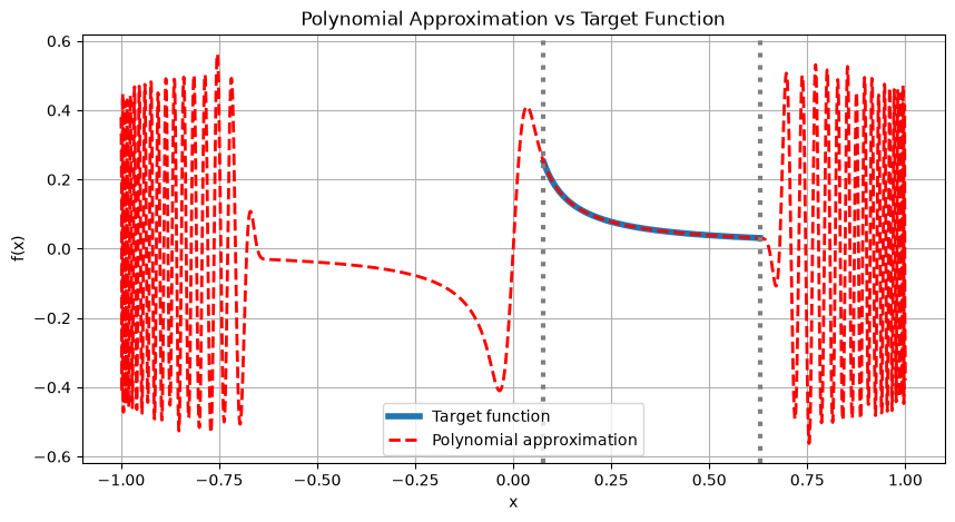
diverges at

x=0

it cannot be bounded by

1

[-1,1]

, so we approximate it only on the range that contains the singular values of the block-encoded operator

A/\alpha

, namely

[\sigma_{\min}/\alpha, \sigma_{\max}/\alpha]

. The target function is

f(x) = \frac{\mathrm{SCALE}}{\kappa_{\rm eff}\, x}, \qquad x\in[\sigma_{\min}/\alpha, \sigma_{\max}/\alpha],

with a factor

\mathrm{SCALE}<1

ensuring

|f(x)|\le 1

(which eases the QSVT angle finding). According to Ref. [2], a degree of

\sim \kappa_{\rm eff} \log(\kappa_{\rm eff}/\epsilon)

suffices to approximate

f

with error

\epsilon

. We use qsp_approximate to fit

f

as a Chebyshev sum bounded by

1

[-1,1]

, and qsvt_phases to obtain the corresponding QSVT phases.

from classiq.applications.qsp import qsp_approximate, qsvt_phases

EPS = 1e-4
SCALE = 0.25

degree = int(kappa_eff * np.log(kappa_eff / EPS))
if degree % 2 == 0:  # inversion requires an odd polynomial
    degree += 1

# Singular values of the block-encoded operator A / alpha.
be_svd = svd / block_encoding.alpha


def target_function(x):
    return SCALE / (kappa_eff * x)


pcoefs, approx_error = qsp_approximate(
    target_function,
    degree=degree,
    parity=1,
    interval=[min(be_svd), max(be_svd)],
    plot=True,
)
inversion_phases = qsvt_phases(pcoefs)

print(f"Polynomial degree: {degree}")
print(f"Max approximation error on the interval: {approx_error}")

Output:

/Users/roiedann/projects/classiq-library/.venv/lib/python3.11/site-packages/classiq/applications/qsp/qsp.py:203: UserWarning: Solution may be inaccurate.

Try another solver, adjusting the solver settings, or solve with verbose=True for more information.
    prob.solve()
  

Output:

Polynomial degree: 151
  Max approximation error on the interval: 5.243390751308308e-07
  

Solving a Linear Equation

Next, we solve an instance of a linear equation

A\vec{x} = \vec{b}

. For this, we define some arbitrary

\vec{b}

vector.

b = np.arange(A_dim)
b_norm = np.linalg.norm(b)
b_normalized = (b / b_norm).tolist()
print(b)

Output:

[0 1 2 3]

Now we build the quantum model. We prepare the initial state

|b\rangle

and then call qsvt_inversion, driving it with the block encoding: the projector marks its block register being zero, its unitary is applied through block_encoding.unitary, and the extra QSVT auxiliary is the last block qubit.

@qfunc
def projector(block: QNum, res: QBit) -> None:
    res ^= block == 0


@qfunc
def main(
    data: Output[QNum[block_encoding.data_size]],
    block: Output[QArray[QBit, block_encoding.block_size + 1]],
) -> None:

    allocate(data)
    allocate(block)
    inplace_prepare_amplitudes(b_normalized, 0, data)

    # QSVT inversion driven by the block encoding: reflect about its block being
    # zero, apply its unitary, and use the last block qubit as the QSVT auxiliary.
    qsvt_inversion(
        phase_seq=inversion_phases,
        block_encoding_cnot=lambda aux: projector(
            block[0 : block_encoding.block_size], aux
        ),
        u=lambda: block_encoding.unitary(data, block[0 : block_encoding.block_size]),
        aux=block[block_encoding.block_size],
    )

Let us synthesize, visualize, and execute. For the execution, we choose a statevector simulator, as we are considering a small problem for demonstrating the algorithm. In addition, later on we would like to verify our result against the expected classical one.

qprog = synthesize(main)
show(qprog)

# Calculate state vector (filter in post-processing)
result = calculate_state_vector(qprog)

Output:


Submitting state-vector job to simulator

Output:

Quantum program link: https://platform.classiq.io/circuit/3K2wIOU7x80TMdTsjnpIy09uRfh
  

If our matrix

A

is block-encoded with a block variable of size

m

, then the QSVT routine block encodes the inverse of

A

m+1

qubits, where the additional qubit is the QSVT auxiliary. Therefore, we need to post-select on block being zero, if we want to obtain a state

\sim A^{-1}|b\rangle

# Filter to block == all zeros (post-select on success)
zero_block = [0] * (block_encoding.block_size + 1)
df = result[result["block"].apply(lambda x: x == zero_block)].sort_values("data")
df

	data	block	amplitude	magnitude	phase	probability	bitstring
56	0	[0, 0, 0, 0, 0]	-0.004095+0.020587j	0.02	0.56π	0.000441	0000000
10	1	[0, 0, 0, 0, 0]	0.024985-0.125607j	0.13	-0.44π	0.016401	0000001
63	2	[0, 0, 0, 0, 0]	0.001560-0.007844j	0.01	-0.44π	0.000064	0000010
24	3	[0, 0, 0, 0, 0]	-0.015714+0.079001j	0.08	0.56π	0.006488	0000011

Comparing to the Expected Result

Finally, we verify our quantum solution, by comparing it to the expected classical one.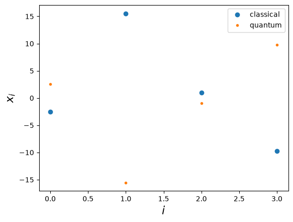

expected_x = np.linalg.inv(A) @ b

After post-selecting the block on zero, the QSVT routine returns

|x\rangle \propto p\!\left(A/\alpha\right)\frac{\vec b}{|\vec b|}, \qquad p\!\left(A/\alpha\right) \approx \frac{\mathrm{SCALE}}{\kappa_{\rm eff}}\left(\frac{A}{\alpha}\right)^{-1} = \frac{\mathrm{SCALE}\,\alpha}{\kappa_{\rm eff}}\,A^{-1}.

Collecting the prefactors — the

\alpha

cancels since

\kappa_{\rm eff}=\alpha\kappa

— the solution is recovered as

\vec x = \frac{|\vec b|\,\kappa}{\mathrm{SCALE}}\,\mathrm{Re}\!\left(\text{amplitudes}\right).

global_phase = np.angle(df.amplitude.iloc[0])
prefactor = b_norm * kappa / SCALE
computed_x = prefactor * np.real(np.array(df.amplitude) / np.exp(1j * global_phase))

Let’s compare it with the expected solution: Comment: even after removing the global phase to ensure a real solution, the quantum solution can be obtained up to a sign.

import matplotlib.pyplot as plt

plt.plot(expected_x, "o", label="classical")
plt.plot(computed_x, ".", label="quantum")
plt.xlabel(r"$i$", fontsize=16)
plt.ylabel(r"$x_i$", fontsize=16)
plt.legend();

assert (
    min(
        np.linalg.norm(computed_x - expected_x),
        np.linalg.norm(-computed_x - expected_x),
    )
    < 0.05
)

One-Line Inversion with `BlockEncoding.inverse`

The implementation above of the inverse (finding the QSVT phases and wiring up qsvt_inversion) is packaged in the BlockEncoding.inverse method. It takes the (bare) condition number and a target precision, forms the effective condition number

\kappa_{\rm eff}=\alpha\kappa

internally, and returns a ready-to-use BlockEncoding of

A^{-1}

. The same linear system is then solved with a single call, reproducing the by-hand result.

be_inverse = block_encoding.inverse(kappa=kappa, eps=1e-2)


# The entry point must be named `main`; this shadows the by-hand `main` above,
# but `qprog` was already synthesized from it and is unaffected.
@qfunc
def main(
    data: Output[QNum[block_encoding.data_size]],
    block: Output[QArray[QBit, be_inverse.block_size]],
) -> None:

    allocate(data)
    allocate(block)
    inplace_prepare_amplitudes(b_normalized, 0, data)
    be_inverse.unitary(data, block)


qprog_direct = synthesize(main)
result_direct = calculate_state_vector(qprog_direct)

zero_block_direct = [0] * be_inverse.block_size
df_direct = result_direct[
    result_direct["block"].apply(lambda x: x == zero_block_direct)
].sort_values("data")

gp_direct = np.angle(df_direct.amplitude.iloc[0])
computed_x_direct = (
    b_norm
    * be_inverse.alpha
    * np.real(np.array(df_direct.amplitude) / np.exp(1j * gp_direct))
)

print("by-hand   :", np.round(computed_x, 3))
print("direct    :", np.round(computed_x_direct, 3))
print("classical :", np.round(expected_x, 3))

Output:


Submitting state-vector job to simulator

Output:

by-hand   : [  2.546 -15.536  -0.97    9.771]
  direct    : [  2.546 -15.536  -0.971   9.771]
  classical : [-2.545 15.536  0.971 -9.771]
  

References

[1]: Martyn JM, Rossi ZM, Tan AK, Chuang IL. Grand unification of quantum algorithms. PRX Quantum 2, 040203. (2021). [2]: A. M. Childs, R. Kothari, and R. D. Somma. Quantum algorithm for systems of linear equations with exponentially improved dependence on precision. SIAM Journal on Computing 46, 1920-1950 (2017).

A Note on Efficient Block-Encoding, Condition Number, and Complexity

An efficient block-encoding of a matrix

A

means that the resources to construct the unitary

U_{A,s}

, as well as the scaling factor

s

, scales poly-logarithmically with the matrix dimension. This technical note concerns the latter point. First, we note that an optimal value for the scaling factor

s

is the maximal singular value

\sigma_{\max}

, namely

s\geq \sigma_{\max}

. This comes directly from the requirement that

||A/s||\leq 1

. For that reason, the effective condition number used throughout the demo,

\kappa = s/\sigma_{\min}

, is bounded from below by the actual condition number

\sigma_{\max}/\sigma_{\min}

. Next, note that if

s

scales linearly with the problem size, then the exponential speedup is lost. This is because the polynomial degree then scales as

O(N)

. In addition, the amplitude of the encoded solution scales the same (although it also depends on the input vector

|b\rangle

), which requires an additional amplitude amplification routine that adds a factor of

O(\sqrt{N})

to the overall resources.

Algorithms

Applications

Tutorials

Matrix Inversion with Quantum Singular Value Transform (QSVT)

View on GitHub

Example: Inverting a Random Matrix

Setting an Example

Block-Encoding

Building the Inverse by Hand with QSVT

Solving a Linear Equation

Comparing to the Expected Result

One-Line Inversion with `BlockEncoding.inverse`

References

A Note on Efficient Block-Encoding, Condition Number, and Complexity

View on GitHub

​Example: Inverting a Random Matrix

​

​Setting an Example

​

​Block-Encoding

​

​Building the Inverse by Hand with QSVT

​

​Solving a Linear Equation

​

​Comparing to the Expected Result

​One-Line Inversion with BlockEncoding.inverse

​References

​A Note on Efficient Block-Encoding, Condition Number, and Complexity

Example: Inverting a Random Matrix

Setting an Example

Block-Encoding

Building the Inverse by Hand with QSVT

Solving a Linear Equation

Comparing to the Expected Result

One-Line Inversion with `BlockEncoding.inverse`

References

A Note on Efficient Block-Encoding, Condition Number, and Complexity