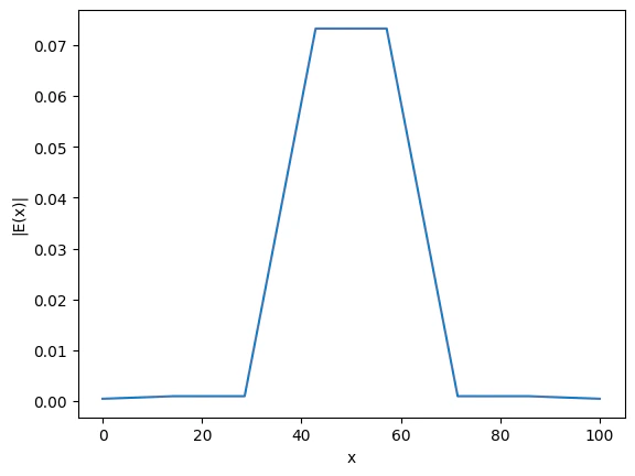
View on GitHub
Open this notebook in GitHub to run it yourself
The Vlasov–Ampère System
We consider a linearized 1D Vlasov–Ampère system with an external driving current. This system governs how perturbations to a background plasma evolve in phase space under the influence of electric fields. The equations are:Physical Meaning and Assumptions
- is the first-order perturbation of the distribution function from equilibrium. It captures how particles deviate from their steady-state behavior: .
- is the (complex) electric field.
- is a known source term (e.g. external driving or antenna).
- encodes non-reflecting boundary conditions:
- for outgoing waves.
- for incoming waves.
- All variables in the equation were normalized such that we get dimensionless equations (see more details in the paper).
Discretizing the variables and leads to very large linear systems. Upon discretization, they form a structured linear system suitable for block encoding, making them compatible with quantum linear solvers. In the next sections, we will show how to construct block encoding for the equations using classiq, then plug it to a linear solver (QSVT in this case) to solve a certain toy problem. We emphasize that due to the dependence of the linear system solver on the condition number - , and the dependece of the condition number in the grid size, we don’t expect any quantum advantage for the 1D system. However, generalizing for higher dimensional systems should be straightforward thanks to the high level modeling approach.
Block Encoding of the linear system
Data encoding
We define a quantum struct that will define the mapping of the coordinates to the effective block-encoded matrix of the problem:v holds the velocity coordinate as a signed number, as the velocity can hold negative values as well.
x holds the position coordinates. It will encode a non-negative number in the range
The value E switches between the encoding of (for E=0) and (for E=1, v=0).
Notice that the values E=1, v!=0 are redundant (in fact we could eliminate them through the projector of the block encoding, but we keep them as they don’t change the reuslt).
Block Struct
We also add additional struct for the block encoding. It will hold additional variables that are required by the encoding process through - for adding block encodings (lcu), eliminating parts of existing block encodings (flag) or for diagonal block encoding (ind).Now we are ready to block encode all parts of the equation. We show how to block encode each part of them, then combine them with Linear Combination of Unitaries. Let us look again on the equations: The matrix we encode will have a row for each ‘s degree of freedom, and a row for each dof. The columns represent the participating terms in each equation.
Block encoding: advective term
Notice that the advective term is in the upper left corner of the block encoded matrix (as it only involves ). Ignoring part, the term is a tensor product of 2 block encodings - a diagonal encoding, and a derivative term.Derivative term
The derivative term consists of normal finite-difference rule intermediate x points. At the boundaries of , the derivative is according to a 2nd order interpolating polynomial (as described in the paper Eqs.19). We decompose it as a sum of 2 matrices: The first matrix is a 1D x-derivative with dirichlet boundary conditions. The 2 diagonals are combined using LCU of modular adders, where the overfolwing terms are eliminated using a flag qubit.x variable to take care for both edges of the system.
It is assumed that the size of x in qubits is at least
Diagonal term
We use theassign_amplitude_table function, that performs the operation , which is exactly a diagonal block encoding, where the additional indicator part of the block qubits.
To save qubits we use implementation for arbitrary , which is not scallable to large variable sizes. However, it is possible to perform it with a linear scaling in the number of qubits, using a primitive that block encodes to the amplitude, using quantum comparator. To achieve the function , one can simply take the square of the block encoding, using qsvt or block encoding multiplication.
For more details, see the qsvt notebook.
Non-reflecting boundary conditions
The term is enforcing non-reflecting boundary conditions, not allowing incoming waves to the system:Block encoding: off diagonal terms
Block encode the force and current terms, corresponding to the upper right and lower left blocks.Loading the force term
In our setting It is a column vector in the matrix, and to load it we have several options. One is to first load one of them ( or as a state, then use amplitude loading of the other one to create a block encoding of the multiplication. A second option that we use here is to directly prepare the state of the multiplication. The advantage is a better scaling factor. It can be performed as suggested here [3] (though for this specific method there would still be a scaling factor issue). For simplicity we use here the general state preparation method (which is not scallable). Finally, we zero the columns for whichv != 0, beacuse we want only columns that encode the field .
Current term
The current term is an integration, represented by row multiplication: To load v, a linear state-preparation is enough. This can be done using the method in [4]. Because we only have equations with this term for the degrees of freedom, we zero columns wherev != 0.
control-else mechanism on the E variable.
We also need to balance both terms to be on the same scaling (both are currently normalized according to the norm of each term), that is done using the function equalize_amplitude.
Full block encoding
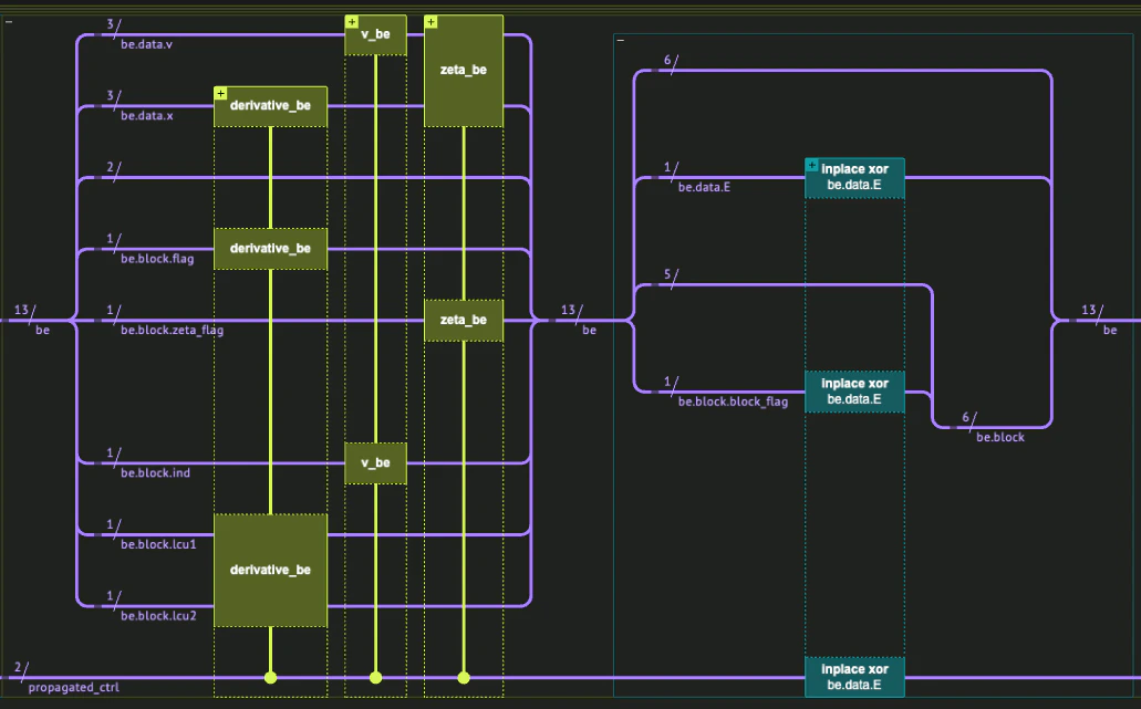
The full block encoding is just a combination of all the terms using LCU. Notice that the diagonal term which has the same coefficient both for and is achieved by simply using theIDENTITY operation (= “do nothing”).
Output:
Extracting the block encoding using quantum simulation
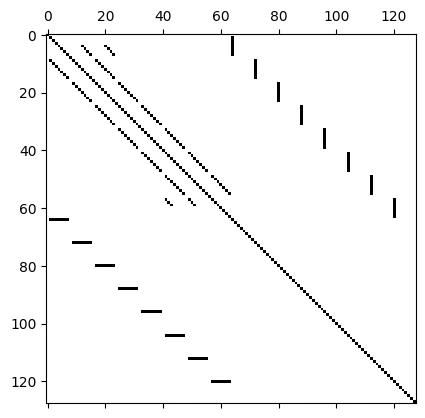
In order to get the resulting block encoded matrix using statevector simulation, we add a reference variable that duplicates the input variable before the application of the block encoding, thus surving as a marker for the input state before the application of the block encoding.Output:
Output:
Linear solver using QSVT matrix inversion
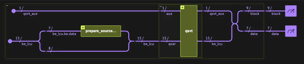
Now we use the block encoding to solve the equation. We only left to encode the external source we want to solve for as initial state, and apply matrix inversion on the it. Because the condition number of the resulting matrix is high for our simulation, we limitied ourselves for small grid size, on which the problem solution is not physical, though we show it for educational purposes.Initial state Loading
We solve for a source term localized at , according to the following formula:QSVT phases calculation
Solve an optimization problem for the qsvt polynomial, and find the corresponding QSVT phases: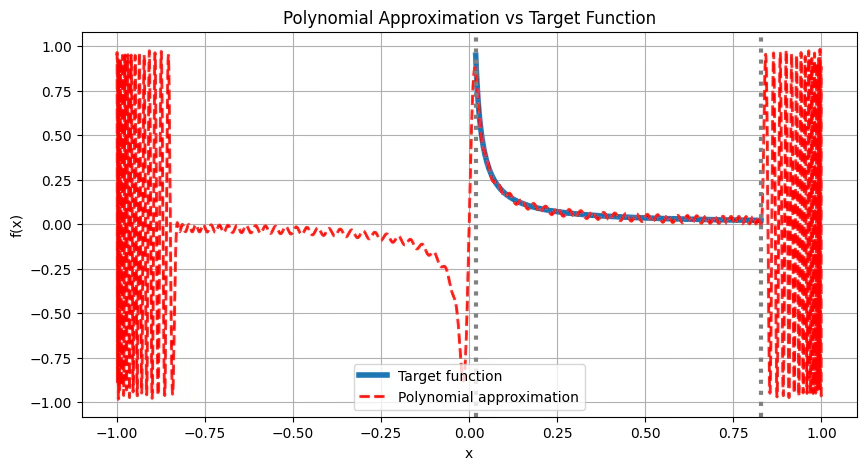
Output:
Full QSVT circuit
Output:
Post-process
| data.v | data.x | data.E | block | amplitude | magnitude | phase | probability | bitstring | |
|---|---|---|---|---|---|---|---|---|---|
| 0 | 1 | 4 | 0 | 0 | 0.013605+0.000471j | 0.01 | 0.01π | 0.000185 | 0000000000001000010 |
| 1 | 1 | 3 | 0 | 0 | 0.013603-0.000472j | 0.01 | -0.01π | 0.000185 | 0000000000000110010 |
| 2 | -4 | 3 | 0 | 0 | 0.007906-0.002675j | 0.01 | -0.10π | 0.000070 | 0000000000000111000 |
| 3 | -4 | 4 | 0 | 0 | 0.007903+0.002675j | 0.01 | 0.10π | 0.000070 | 0000000000001001000 |
| 4 | -3 | 4 | 0 | 0 | 0.005077+0.002067j | 0.01 | 0.12π | 0.000030 | 0000000000001001010 |
| 5 | -3 | 3 | 0 | 0 | 0.005076-0.002069j | 0.01 | -0.12π | 0.000030 | 0000000000000111010 |
| 6 | 2 | 4 | 0 | 0 | 0.003209-0.000324j | 0.00 | -0.03π | 0.000010 | 0000000000001000100 |
| 7 | 2 | 3 | 0 | 0 | 0.003206+0.000325j | 0.00 | 0.03π | 0.000010 | 0000000000000110100 |
| 8 | 0 | 2 | 1 | 0 | 0.001109+0.000937j | 0.00 | 0.22π | 0.000002 | 0000000000010100000 |
| 9 | 0 | 3 | 1 | 0 | 0.001104+0.049842j | 0.05 | 0.49π | 0.002485 | 0000000000010110000 |
Output:
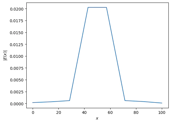
Compare to a classical solver
Output: