

View on GitHub
Open this notebook in GitHub to run it yourself
Welcome to the Jungle of HHL
- Rabbits vs.
Lanchester Model
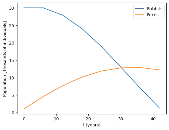
Lanchester Model is described in this link. This differential equation describes the behavior of two forces, and : where the coefficients described in the next sections indicate the sensitivities of each side to the other and to itself.Describing the Classical Model Using the Finite Difference Method
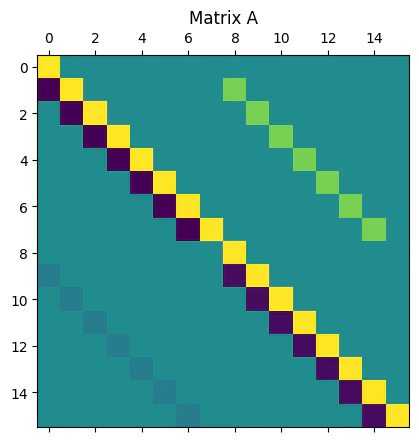
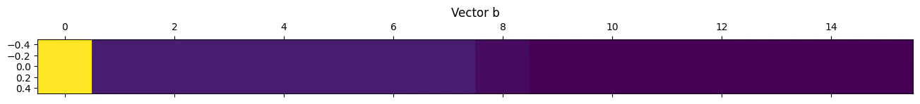
Assuming , : where the dot product was added explicitly to emphasize that is a variable. The first sample is the initial condition: Then, for any next point, we solve numerically using the previous point: The system of linear equations describing the model looks like this:Building the Matrix with NumPy
- () and () define the rate of natural losses or birth (due to death, disease, etc.).
- () and () define the rate of losses due to environmental factors (affecting both species).
- () and () are losses or gains due to interactions between species (prey hunted by predators and vice versa).
- () and () are gains due to migration.
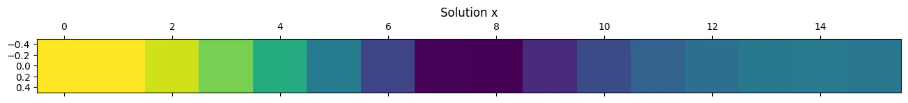
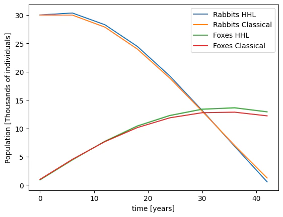
Classical Solution
Redefining the Matrix
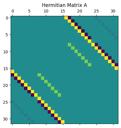
The matrix of HHL is a canonical one, assuming the following properties:- The RHS vector is normalized.
- The matrix is a Hermitian one.
- The matrix is of size .
- The eigenvalues of are in the range .
1) Normalized b
As preprocessing, normalize and then return the normalization factor as postprocessing.2) Hermitian Matrix
Symmetrize the problem: This increases the number of qubits by
3) Make the Matrix of Size
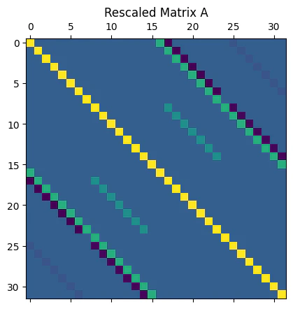
Complete the matrix dimension to the closest with an identity matrix. The vector is completed with zeros. However, our matrix is already the right size.4) Rescaled Matrix
If the eigenvalues of are in the range , we can employ transformations to the exponentiated matrix and then undo them to extract the results: The eigenvalues of this matrix lie in the interval , and are related to the eigenvalues of the original matrix via with being an eigenvalue of resulting from the QPE algorithm. This relation between eigenvalues is then used for the expression inserted into the eigenvalue inversion, via theAmplitudeLoading function.
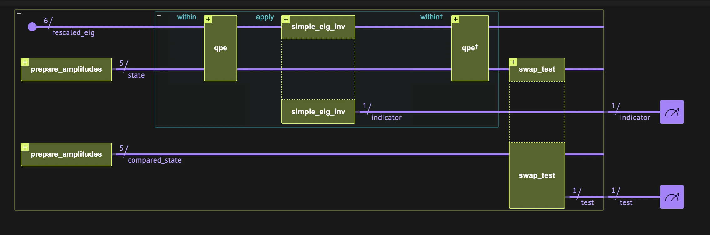
Defining HHL Algorithm for the Quantum Solution
This section is based on Classiq HHL in the user guide, here and here. Note the rescaling insimple_eig_inv based on the matrix rescaling.
Synthesize and Show
Output:
Execution and Results Analysis
The analysis is explained in the swap test user guide. We compare the measured overlap with the exact overlap using the expected probability of measuring the state , defined as We extract the overlap . The exact overlap is computed with the dot product of the two state vectors. Note that for the sake of this demonstration we execute this circuit times to improve the precision of the probability estimate. This is usually not required. Since we are in the HHL context, we filter only theindicator==1 results.
Output:
indicator=1 results, the bar of test=0 is much higher than test=1.
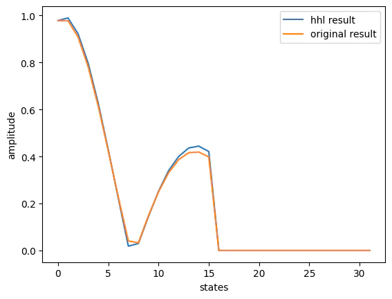
State Vector Simulation
We can also run the state vector of the HHL result and examine it without a swap test. Extracting the full information is exponentially hard, and used here just for educational purposes. Extension of this work can extract some information from the state vector, such as the last element, which is the most important. We can also pad the last solution with an extension, and therefore measure the last point with high probability.Output:
indicator=1 and phase=0 results.
Output: