

View on GitHub
Open this notebook in GitHub to run it yourself
Building a Geometric Brownian Motion (GBM) Price Model — from Analytic Formula to Quantum Circuit
Motivation
Pricing path-dependent derivatives such as Asian options often requires evaluating a Geometric Brownian Motion (GBM) over many time steps.- Classical approach: Monte Carlo simulation over many paths and timesteps.
- Quantum approach:
- Compress the representation of randomness (load distributions into amplitudes).
- Achieve a quadratic speed-up for expectation estimation via Quantum Amplitude Estimation (QAE).
- Derive a Chebyshev-truncated Karhunen–Loève (KL) expansion.
- Convert that expansion to Classiq quantum arithmetic.
- Synthesize hardware-aware circuits for multiple targets with a single command.
- Chebyshev Polynomials in the KL Expansion
KL expansion (Chebyshev-truncated form)
The KL expansion expresses as an orthogonal sine series with i.i.d. Gaussian coefficients . In truncated form: where are Chebyshev polynomials of the second kind.Gaussian discretization (classical preprocessing)
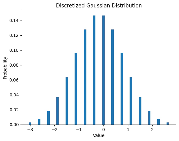
Goal: build a discrete approximation of a Gaussian distribution so that its probabilities can be loaded into amplitudes. Typical steps:- Select range (e.g., standard deviations).
- Use bins for qubits.
- Compute bin probabilities using the Gaussian CDF:
- Normalize the probability vector so .
- A list of grid points (bin edges or centers)
- A probability vector suitable for amplitude loading.
Quantum function approximation for and
For simplicity in the demo:- Implement and via low-order Taylor-like polynomials (around ).
- This keeps the arithmetic shallow and highlights the modeling flow.
- After preparing a superposition over , the computed value register becomes entangled with , representing a function evaluation “in parallel worlds.”
Output:
Output:
Output:
Chebyshev Polynomials
The Chebyshev polynomials are a sequence of orthogonal polynomials that are related to de Moivre’s formula and the trigonometric functions. They are defined by the recurrence relation:- Loop depth grows as .
- Doubling truncation order increases gate count only linearly (hardware-friendly).
Output:
Output:
Brownian Motion
The Brownian motion is a stochastic process that models the random movement of particles in a fluid. The approximate solution in this context is the truncated Wiener series. Key ingredients in the quantum model:- Prepare registers for coefficients (a_0,\dots,a_{L-1}) from the discretized Gaussian distribution (amplitude loading).
- Prepare a time register (t) in superposition (e.g., Hadamards over a time index).
- Compute:
- (or a stand-in approximation)
- (or a stand-in approximation)
- via recurrence
- Accumulate the weighted sum to form .
Return-to-price space (GBM mapping)
Convert (log-)returns to price using the GBM form: In the demo notebook :- Exponentiation may be implemented via a simple approximation for .
- More accurate quantum exponentiation methods exist in the literature (see referenced suggestions in https://arxiv.org/pdf/2001.00807.pdf for example).
Putting it all together
Output:
Output:
Output:
Final reflection and quantum roadmap
This notebook illustrates that a mathematically heavy model (KL-truncated GBM + Chebyshev recursion) becomes circuit-light once randomness is moved into amplitudes. Next steps toward pricing (expected payoff):- Amplitude loading: put Gaussian coefficients into superposition with gates (matching the power-of-two grid).
- Nested QAE (conceptually):
- First QAE estimates time-averaged price along the path.
- Second QAE wraps the payoff.
- Query complexity can still beat classical Monte Carlo scaling.
- Potential shortcut (as hinted in the reference):
- Drop one QAE via smart time subsampling to reduce depth without extra qubits (constants and practical tradeoffs depend on implementation details).
- The classical formula is algebraically dense, but the quantum program is highly structured, enabling modeling-focused development with automated circuit synthesis.